Downstream analysis for multi-group analysis
XSun
2025-01-07
Last updated: 2025-01-23
Checks: 6 1
Knit directory: multigroup_ctwas_analysis/
This reproducible R Markdown analysis was created with workflowr (version 1.7.0). The Checks tab describes the reproducibility checks that were applied when the results were created. The Past versions tab lists the development history.
The R Markdown file has unstaged changes. To know which version of
the R Markdown file created these results, you’ll want to first commit
it to the Git repo. If you’re still working on the analysis, you can
ignore this warning. When you’re finished, you can run
wflow_publish to commit the R Markdown file and build the
HTML.
Great job! The global environment was empty. Objects defined in the global environment can affect the analysis in your R Markdown file in unknown ways. For reproduciblity it’s best to always run the code in an empty environment.
The command set.seed(20231112) was run prior to running
the code in the R Markdown file. Setting a seed ensures that any results
that rely on randomness, e.g. subsampling or permutations, are
reproducible.
Great job! Recording the operating system, R version, and package versions is critical for reproducibility.
Nice! There were no cached chunks for this analysis, so you can be confident that you successfully produced the results during this run.
Great job! Using relative paths to the files within your workflowr project makes it easier to run your code on other machines.
Great! You are using Git for version control. Tracking code development and connecting the code version to the results is critical for reproducibility.
The results in this page were generated with repository version 6c7c5cb. See the Past versions tab to see a history of the changes made to the R Markdown and HTML files.
Note that you need to be careful to ensure that all relevant files for
the analysis have been committed to Git prior to generating the results
(you can use wflow_publish or
wflow_git_commit). workflowr only checks the R Markdown
file, but you know if there are other scripts or data files that it
depends on. Below is the status of the Git repository when the results
were generated:
Ignored files:
    Ignored:    .Rhistory

Unstaged changes:
    Modified:   analysis/multi_group_downstream_analysis.Rmd
Note that any generated files, e.g. HTML, png, CSS, etc., are not included in this status report because it is ok for generated content to have uncommitted changes.
These are the previous versions of the repository in which changes were
made to the R Markdown
(analysis/multi_group_downstream_analysis.Rmd) and HTML
(docs/multi_group_downstream_analysis.html) files. If
you’ve configured a remote Git repository (see
?wflow_git_remote), click on the hyperlinks in the table
below to view the files as they were in that past version.
| File | Version | Author | Date | Message |
|---|---|---|---|---|
| Rmd | 6c7c5cb | XSun | 2025-01-22 | update |
| html | 6c7c5cb | XSun | 2025-01-22 | update |
| Rmd | 0189bd3 | XSun | 2025-01-22 | update |
| Rmd | cfed192 | XSun | 2025-01-17 | update |
| html | cfed192 | XSun | 2025-01-17 | update |
| Rmd | d47a369 | XSun | 2025-01-17 | update |
| html | d47a369 | XSun | 2025-01-17 | update |
| Rmd | 25aaa64 | XSun | 2025-01-15 | update |
| html | 25aaa64 | XSun | 2025-01-15 | update |
| Rmd | 10833df | XSun | 2025-01-14 | update |
| Rmd | c432d5f | XSun | 2025-01-12 | update |
| html | c432d5f | XSun | 2025-01-12 | update |
| Rmd | 8692522 | XSun | 2025-01-11 | update |
| html | 8692522 | XSun | 2025-01-11 | update |
| Rmd | 6bf3c77 | XSun | 2025-01-10 | update |
| html | 6bf3c77 | XSun | 2025-01-10 | update |
| Rmd | 80e204a | XSun | 2025-01-10 | update |
| html | 80e204a | XSun | 2025-01-10 | update |
library(ctwas)
library(ggplot2)
library(dplyr)
library(tidyr)
library(gridExtra)
library(pheatmap)
library(VennDiagram)

source("/project/xinhe/xsun/multi_group_ctwas/data/selected_tissues.R")
source("/project/xinhe/xsun/multi_group_ctwas/data/samplesize.R")

mapping_predictdb <- readRDS("/project2/xinhe/shared_data/multigroup_ctwas/weights/mapping_files/PredictDB_mapping.RDS")
mapping_munro <- readRDS("/project2/xinhe/shared_data/multigroup_ctwas/weights/mapping_files/Munro_mapping.RDS")
mapping_two <- rbind(mapping_predictdb,mapping_munro)

traits <- names(tissues_alltraits)
traits <- traits[order(traits)]

brain_traits <- c("ASD-ieu-a-1185","BIP-ieu-b-5110","MDD-ieu-b-102","NS-ukb-a-230","PD-ieu-b-7","SCZ-ieu-b-5102")


create_bubble_plot <- function(trait, param, gwas_n, tissue_order) {

  ctwas_parameters <- summarize_param(param, gwas_n)

  # Extract and process PVE data
  prop_pve <- ctwas_parameters$prop_heritability
  prop_pve_df <- data.frame(
    Tissue = sapply(strsplit(names(prop_pve), "\\|"), `[`, 1),
    QTL = sapply(strsplit(names(prop_pve), "\\|"), `[`, 2),
    Value = prop_pve
  )
  prop_pve_matrix <- as.data.frame(pivot_wider(prop_pve_df, names_from = QTL, values_from = Value))
  prop_pve_matrix <- prop_pve_matrix[-which(prop_pve_matrix$Tissue == "SNP"),]
  prop_pve_matrix <- prop_pve_matrix[,-which(colnames(prop_pve_matrix) == "NA")]

  # Extract and process enrichment data
  enrich <- ctwas_parameters$enrichment
  enrich_df <- data.frame(
    Tissue = sapply(strsplit(names(enrich), "\\|"), `[`, 1),
    QTL = sapply(strsplit(names(enrich), "\\|"), `[`, 2),
    Value = enrich
  )
  enrich_matrix <- as.data.frame(pivot_wider(enrich_df, names_from = QTL, values_from = Value))

  # Convert matrices to long format and merge
  pve_long <- prop_pve_matrix %>%
    pivot_longer(cols = -Tissue, names_to = "Trait", values_to = "prop_PVE")
  enrich_long <- enrich_matrix %>%
    pivot_longer(cols = -Tissue, names_to = "Trait", values_to = "Enrichment")

  plot_data <- left_join(pve_long, enrich_long, by = c("Tissue", "Trait"))
  plot_data$Tissue <- gsub(pattern = "_", replacement = " ", x = plot_data$Tissue)
  plot_data <- plot_data %>%
    mutate(prop_PVE = prop_PVE * 100)
  #plot_data$Tissue <- factor(plot_data$Tissue, levels = unique(plot_data$Tissue))
  plot_data$Tissue <- factor(plot_data$Tissue, levels = rev(unique(plot_data$Tissue)))

  # Create the bubble plot
  p <- ggplot(plot_data, aes(x = Trait, y = Tissue, size = prop_PVE, color = Enrichment)) +
    geom_point(alpha = 0.7) +
    scale_size(range = c(1, 20), name = "Percentage of Heritability (%)") +
    scale_color_gradient(low = "lightblue", high = "darkblue", name = "Enrichment") +
    labs(x = "Modalities", y = "Tissues") +
    guides(size = guide_legend(override.aes = list(color = "lightblue"))) +
    ggtitle(trait) +
    theme_minimal() +
    theme(
      axis.text.x = element_text(size = 16, angle = 45, hjust = 1),
      axis.text.y = element_text(size = 16),
      axis.title.x = element_text(size = 16),
      axis.title.y = element_text(size = 16),
      legend.text = element_text(size = 16),
      legend.title = element_text(size = 18)
    )

  return(p)
}

plot_heatmap_bytissue <- function(heatmap_data, main, tissues) {

  rownames(heatmap_data) <- heatmap_data$gene_name
  heatmap_data <- heatmap_data %>% dplyr::select(-gene_name, -combined_pip)

  pip_types <- c("|eQTL_pip", "|sQTL_pip", "|stQTL_pip")

  combinations <- expand.grid(pip_types, tissues)
  order <- paste0(combinations$Var2, combinations$Var1)

  heatmap_data <- heatmap_data[,order]

  if(nrow(heatmap_data) ==1){

    heatmap_data <- rbind(heatmap_data,rep(0,ncol(heatmap_data)))
    rownames(heatmap_data)[2] <- "fake_gene_for_plotting"

  }

  heatmap_matrix <- as.matrix(heatmap_data)

  p <- pheatmap(heatmap_matrix,
                cluster_rows = F,   # Cluster the rows (genes)
                cluster_cols = F,   # Cluster the columns (QTL types)
                color = colorRampPalette(c("white", "red"))(50), # Color gradient
                display_numbers = TRUE, # Display numbers in cells
                main = main,labels_row = rownames(heatmap_data), silent = T)

  return(p)
}

plot_heatmap_byomics <- function(heatmap_data, main) {

  rownames(heatmap_data) <- heatmap_data$gene_name
  heatmap_data <- heatmap_data %>% dplyr::select(-gene_name, -combined_pip)

  if(nrow(heatmap_data) ==1){

    heatmap_data <- rbind(heatmap_data,rep(0,ncol(heatmap_data)))
    rownames(heatmap_data)[2] <- "fake_gene_for_plotting"

  }

  heatmap_matrix <- as.matrix(heatmap_data)

  p <- pheatmap(heatmap_matrix,
                cluster_rows = F,   # Cluster the rows (genes)
                cluster_cols = F,   # Cluster the columns (QTL types)
                color = colorRampPalette(c("white", "red"))(50), # Color gradient
                display_numbers = TRUE, # Display numbers in cells
                main = main,labels_row = rownames(heatmap_data), silent = T)

  return(p)
}
Setting1: variance shared by the same QTLs
Parameters
folder_results <- "/project/xinhe/shengqian/ctwas_GWAS_analysis/results/"

all_var <-c()
for(trait in traits[!traits %in% brain_traits]){

  param <- readRDS(paste0(folder_results, "/", trait, "/", trait, ".param.RDS"))
  gwas_n <- samplesize[trait]

  ctwas_parameters <- summarize_param(param, gwas_n)

  var <- cbind(names(ctwas_parameters$group_prior_var),ctwas_parameters$group_prior_var)
  colnames(var) <- c(paste0(trait,"_tissues"), paste0(trait,"_variance"))

  all_var <- cbind(all_var, var)
}

rownames(all_var) <- seq(1:nrow(all_var))

DT::datatable(all_var,caption = htmltools::tags$caption( style = 'caption-side: left; text-align: left; color:black;  font-size:150% ;','Variance for each group, non-psychiatric traits'),options = list(pageLength = 20) )
all_var <-c()
for(trait in brain_traits){
param <- readRDS(paste0(folder_results, "/", trait, "/", trait, ".param.RDS"))
gwas_n <- samplesize[trait]
ctwas_parameters <- summarize_param(param, gwas_n)
var <- cbind(names(ctwas_parameters$group_prior_var),ctwas_parameters$group_prior_var)
colnames(var) <- c(paste0(trait,"_tissues"), paste0(trait,"_variance"))
all_var <- cbind(all_var, var)
}
rownames(all_var) <- seq(1:nrow(all_var))
DT::datatable(all_var,caption = htmltools::tags$caption( style = 'caption-side: left; text-align: left; color:black; font-size:150% ;','Variance for each group, psychiatric traits'),options = list(pageLength = 20) )Genetic architecture of complex traits
Bubble plot: h2g partition across tissues and omics
Tissue order is from: https://sq-96.github.io/multigroup_ctwas_analysis/GWAS_tissue_selection.html
folder_results <- "/project/xinhe/shengqian/ctwas_GWAS_analysis/results/"

p <- list()
for(trait in traits[!traits %in% brain_traits]){

  param <- readRDS(paste0(folder_results, "/", trait, "/", trait, ".param.RDS"))
  gwas_n <- samplesize[trait]
  tissue_order <- tissues_alltraits[[trait]]
  p[[length(p)+1]] <- create_bubble_plot(trait = trait,param = param,gwas_n = gwas_n, tissue_order = tissue_order)

}

print("Non-psychiatric")
[1] "Non-psychiatric"grid.arrange(grobs = p, ncol = 3, nrow = 5)
folder_results <- "/project/xinhe/shengqian/ctwas_GWAS_analysis/results/"

p <- list()
for(trait in brain_traits){

  param <- readRDS(paste0(folder_results, "/", trait, "/", trait, ".param.RDS"))
  gwas_n <- samplesize[trait]
  tissue_order <- tissues_alltraits[[trait]]
  p[[length(p)+1]] <- create_bubble_plot(trait = trait,param = param,gwas_n = gwas_n, tissue_order = tissue_order)

}

print("psychiatric")
[1] "psychiatric"grid.arrange(grobs = p, ncol = 3, nrow = 2)
The power of gene discovery
load("/project/xinhe/xsun/multi_group_ctwas/13.post_processing_0103/results_downstream/compare_multi_single_genenum.rdata")

sum <- sum[!sum$trait %in% brain_traits,]

sum$num_multi <- as.numeric(sum$num_multi)
sum$num_single <- as.numeric(sum$num_single)
sum$overlap <- as.numeric(sum$overlap)
#sum$overlap_adj <- as.numeric(sum$overlap) * 1.001   # Adjust the value to slightly offset behind the main bars

data_long <- pivot_longer(sum, cols = c(num_single, num_multi), names_to = "category", values_to = "count")

print("Non-psychiatric")
[1] "Non-psychiatric"# Facet by trait, with tissues as the bars
ggplot(data_long, aes(x = tissue_single, y = count, fill = category)) +
geom_bar(stat = "identity", position = position_dodge(width = 0.8), width = 0.8) +
geom_bar(data = sum, aes(x = tissue_single, y = overlap), stat = "identity", position = position_dodge(width = 0.8), fill = "grey", alpha = 0.7, width = 0.8) +
facet_wrap(~ trait, nrow = 1, scales = "free_x") + # Display all facets in one row with free scales on x
labs(x = "Tissue", y = "Number of Significant Genes") +
scale_fill_manual(values = c("num_single" = "skyblue", "num_multi" = "orange")) +
theme_minimal() +
theme(axis.text.x = element_text(size = 12, angle = 45, vjust = 0.7, hjust = 0.6), # Adjusted hjust here
axis.text.y = element_text(size = 12),
axis.title.x = element_text(size = 14),
axis.title.y = element_text(size = 14),
strip.background = element_blank(),
strip.text.x = element_text(size = 12, face = "bold"))
load("/project/xinhe/xsun/multi_group_ctwas/13.post_processing_0103/results_downstream/compare_multi_single_genenum.rdata")

sum <- sum[sum$trait %in% brain_traits,]

sum$num_multi <- as.numeric(sum$num_multi)
sum$num_single <- as.numeric(sum$num_single)
sum$overlap <- as.numeric(sum$overlap)
#sum$overlap_adj <- as.numeric(sum$overlap) * 1.001   # Adjust the value to slightly offset behind the main bars

data_long <- pivot_longer(sum, cols = c(num_single, num_multi), names_to = "category", values_to = "count")

print("psychiatric")
[1] "psychiatric"# Facet by trait, with tissues as the bars
ggplot(data_long, aes(x = tissue_single, y = count, fill = category)) +
geom_bar(stat = "identity", position = position_dodge(width = 0.8), width = 0.8) +
geom_bar(data = sum, aes(x = tissue_single, y = overlap), stat = "identity", position = position_dodge(width = 0.8), fill = "grey", alpha = 0.7, width = 0.8) +
facet_wrap(~ trait, nrow = 1, scales = "free_x") + # Display all facets in one row with free scales on x
labs(x = "Tissue", y = "Number of Significant Genes") +
scale_fill_manual(values = c("num_single" = "skyblue", "num_multi" = "orange")) +
theme_minimal() +
theme(axis.text.x = element_text(size = 12, angle = 45, vjust = 0.7, hjust = 0.6), # Adjusted hjust here
axis.text.y = element_text(size = 12),
axis.title.x = element_text(size = 14),
axis.title.y = element_text(size = 14),
strip.background = element_blank(),
strip.text.x = element_text(size = 12, face = "bold"))
SCZ-ieu-b-5102
trait <- "SCZ-ieu-b-5102"

folder_results_multi <- "/project/xinhe/shengqian/ctwas_GWAS_analysis/results/"
folder_results_single <- "/project/xinhe/shengqian/single_tissue_screen/processed_weights/expression_weights/"
tissue_single <- "Brain_Hippocampus"

combined_pip_by_group_multi <- readRDS(paste0(folder_results_multi,trait,"/",trait,".combined_pip_bygroup_final.RDS"))
combined_pip_by_group_single <- readRDS(paste0(folder_results_single,trait,"/",trait,"_",tissue_single,".combined_pip_bygroup_final.RDS"))

combined_pip_by_group_sig_multi <- combined_pip_by_group_multi[combined_pip_by_group_multi$combined_pip > 0.8,]
combined_pip_by_group_sig_single <- combined_pip_by_group_single[combined_pip_by_group_single$combined_pip > 0.8,]

overlap <- combined_pip_by_group_sig_multi[combined_pip_by_group_sig_multi$gene_name %in% combined_pip_by_group_sig_single$gene_name,]

sprintf("# of unique genes from multi-group analysis = %s", nrow(combined_pip_by_group_sig_multi))
[1] "# of unique genes from multi-group analysis = 28"sprintf("# of unique genes from single-group analysis = %s", nrow(combined_pip_by_group_sig_single))[1] "# of unique genes from single-group analysis = 16"sprintf("# of overlapped genes = %s", nrow(overlap))[1] "# of overlapped genes = 4"plot_heatmap_byomics(heatmap_data = combined_pip_by_group_sig_multi[!combined_pip_by_group_sig_multi$gene_name %in% combined_pip_by_group_sig_single$gene_name,], main = "PIP partition for unique genes with PIP > 0.8 from multi-group analysis")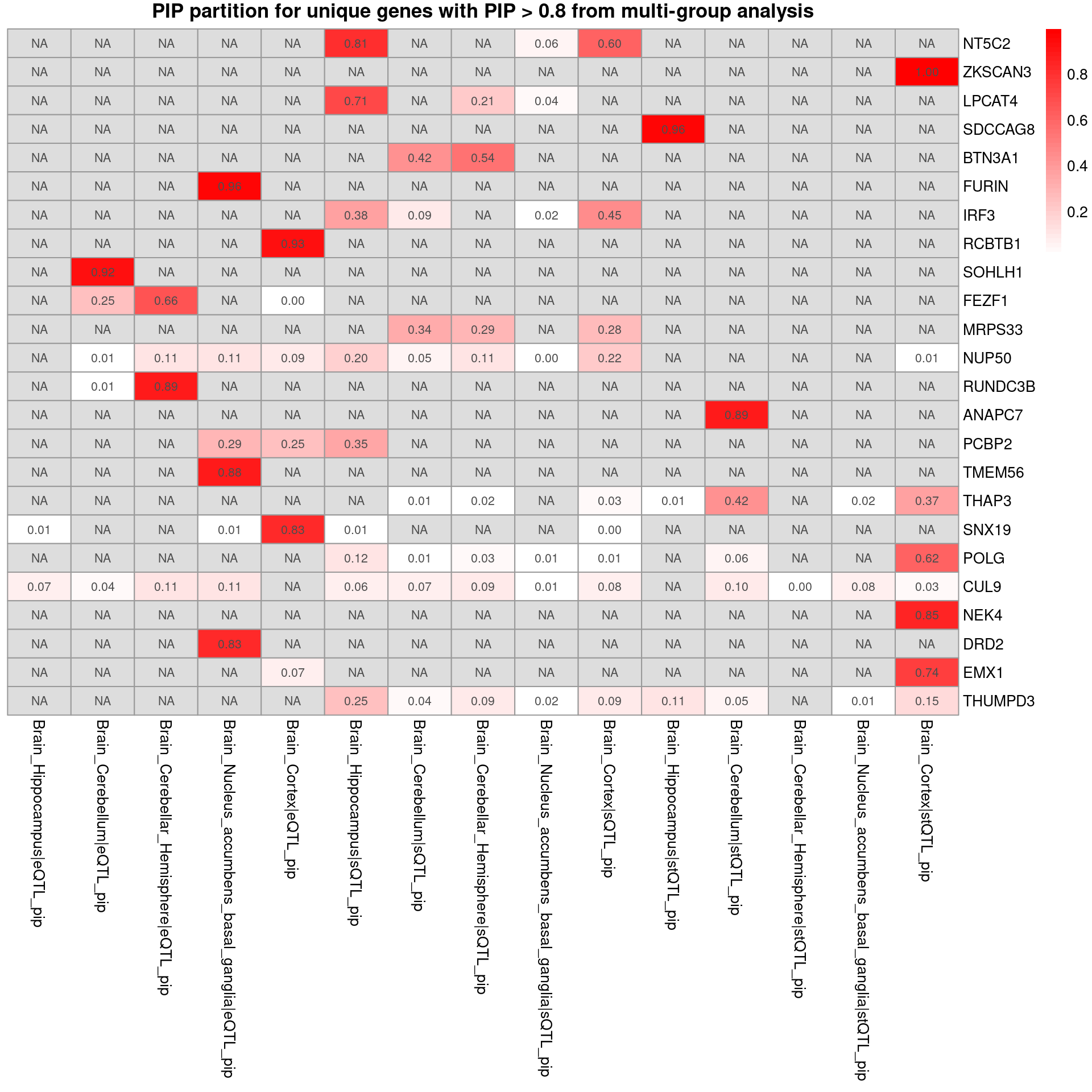
plot_heatmap_byomics(heatmap_data = combined_pip_by_group_sig_multi[combined_pip_by_group_sig_multi$gene_name %in% combined_pip_by_group_sig_single$gene_name,], main = "PIP partition for overlapped genes ")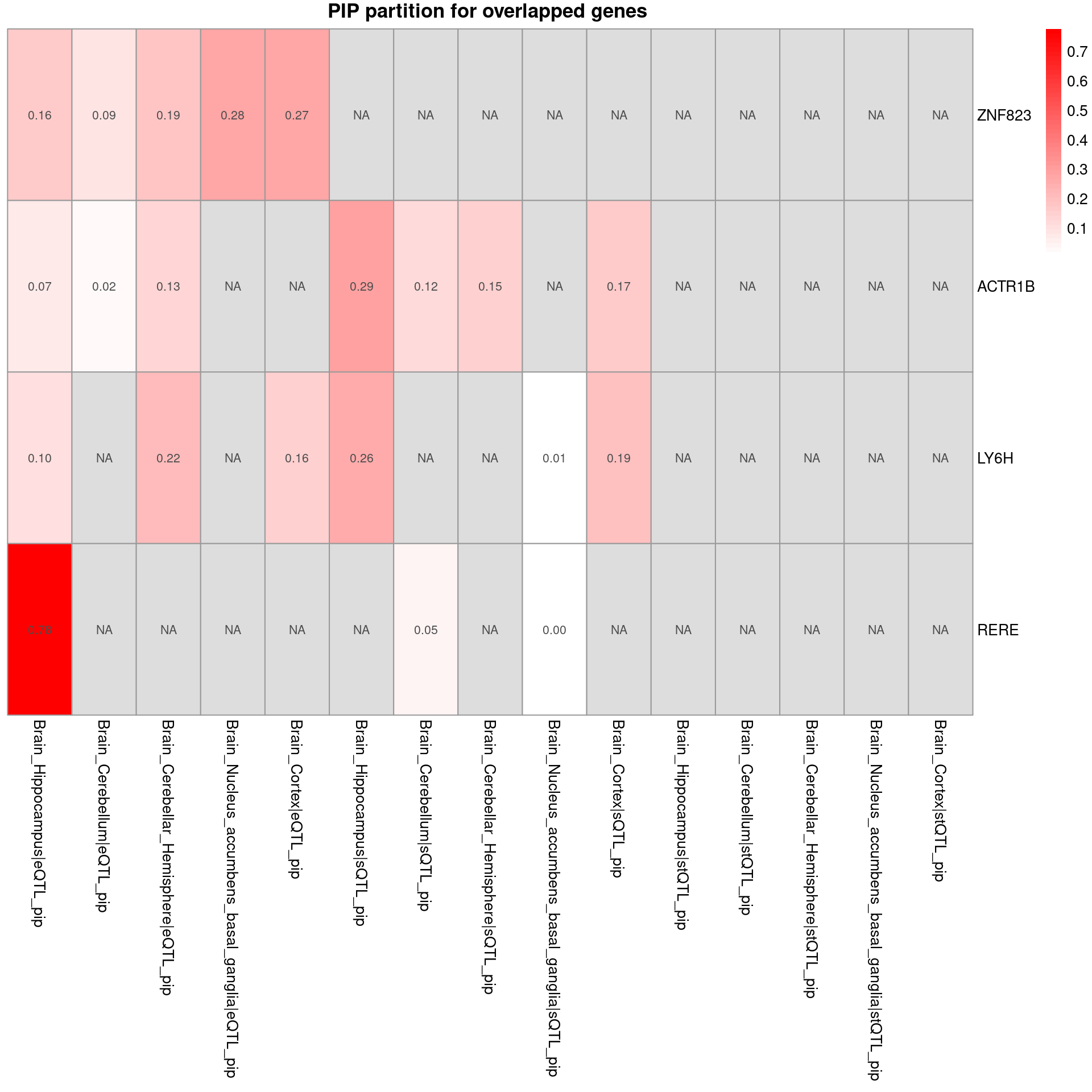
| Version | Author | Date |
|---|---|---|
| 8692522 | XSun | 2025-01-11 |
DT::datatable(combined_pip_by_group_sig_single[!combined_pip_by_group_sig_single$gene_name %in% combined_pip_by_group_sig_multi$gene_name,],caption = htmltools::tags$caption( style = 'caption-side: left; text-align: left; color:black; font-size:150% ;','Unique genes from single eqtl analysis'),options = list(pageLength = 10) )- Among the single eQTL unique genes, HIST1H2BN and HLA-DMB may relate to SCZ
- Among the multi-group unique genes, NT5C2, DRD2,SDCCAG8 may relate to SCZ
- Among the overlapped genes, RERE may relate to SCZ
Highlight the causal context and modality
For all: https://drive.google.com/drive/folders/1COItzR1y_Em6UXb_J8XCzqP-PuXIth6J?usp=share_link
MDD-ieu-b-102
trait <- "MDD-ieu-b-102"

combined_pip_multi <- readRDS(paste0("/project/xinhe/shengqian/ctwas_GWAS_analysis/results/",trait,"/",trait,".combined_pip_bygroup_final.RDS"))
combined_pip_sig_multi <- combined_pip_multi[combined_pip_multi$combined_pip > 0.8,]

# plot_heatmap_bytissue(heatmap_data = combined_pip_sig_multi, main = "PIP partition for genes with PIP > 0.8 from multi-group analysis",tissues = tissues_alltraits[[trait]])
plot_heatmap_byomics(heatmap_data = combined_pip_sig_multi, main = "PIP partition for genes with PIP > 0.8 from multi-group analysis")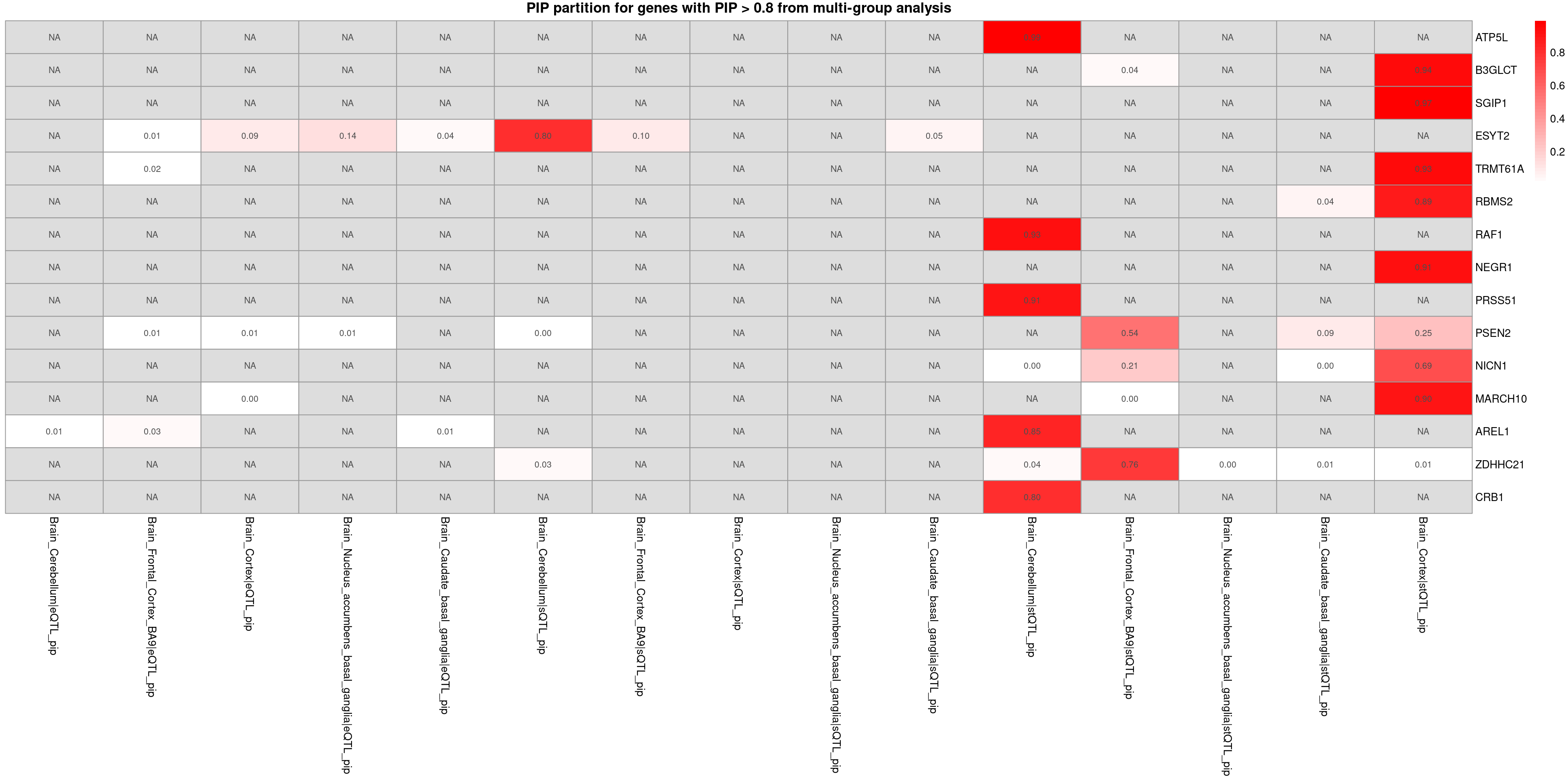
Notes from chatgpt
- NEGR1: Known to be associated with neurodevelopmental processes and has been implicated in GWAS studies for depression and related traits.
- PSEN2: While primarily associated with Alzheimer’s disease, some studies suggest its involvement in mood disorders due to its role in neural processes.
- RAF1: Involved in MAPK/ERK signaling pathways, which can influence stress responses and mood regulation.
Explore allelic heterogeneity (AH)
load("/project/xinhe/xsun/multi_group_ctwas/13.post_processing_0103/results_downstream/pip_per_cs_alltraits.rdata")
DT::datatable(pip_per_cs_alltraits,caption = htmltools::tags$caption( style = 'caption-side: left; text-align: left; color:black;  font-size:150% ;','PIP per CS, for genes with AH'),options = list(pageLength = 10) )
Notes from chatgpt:
LDL:
- SNX17 (Sorting Nexin 17):
- Function: SNX17 is involved in endocytic recycling and intracellular trafficking.
- Relevance to LDL: SNX17 interacts with LDL receptor-related proteins and plays a role in recycling LDL receptors to the cell surface. It has been implicated in maintaining LDL receptor homeostasis, making it relevant to LDL metabolism.
- ABCA1 (ATP Binding Cassette Subfamily A Member 1):
- Function: ABCA1 is critical in cholesterol efflux, facilitating the transfer of cholesterol to HDL particles.
- Relevance to LDL: ABCA1 indirectly influences LDL levels by regulating cholesterol homeostasis and promoting reverse cholesterol transport. Variants in ABCA1 are strongly associated with lipid metabolism disorders.
Reduce FP findings
Silver standard for T2D LDL BMI RBC IBD – summary
traits_used_in_silver <- c("T2D-panukb","LDL-ukb-d-30780_irnt","BMI-panukb","RBC-panukb","IBD-ebi-a-GCST004131")
traits_silver <- c("T2D","LDL","BMI","RBC","IBD")
top_tissues <- c("Pituitary","Liver","Cells_Cultured_fibroblasts","Skin_Not_Sun_Exposed_Suprapubic","Whole_Blood")
names(top_tissues) <- c("T2D-panukb","LDL-ukb-d-30780_irnt","BMI-panukb","RBC-panukb","IBD-ebi-a-GCST004131")

folder_single_results <- "/project/xinhe/shengqian/single_tissue_screen/processed_weights/expression_weights/"
folder_multi_results <- "/project/xinhe/shengqian/ctwas_GWAS_analysis/results/"

stats_all <- c()
stats_all_twas <- c()
p <- list()
for (i in 1:length(traits_used_in_silver)){


  known <- readRDS(paste0("/project/xinhe/xsun/multi_group_ctwas/data/silverstandard/known_annotations_",traits_silver[i],".RDS"))
  bystander <- readRDS(paste0("/project/xinhe/xsun/multi_group_ctwas/data/silverstandard/bystanders_",traits_silver[i],".RDS"))

  # single group results

  tissue <- top_tissues[traits_used_in_silver[i]]

  z_gene_single <-readRDS(paste0(folder_single_results,"/",traits_used_in_silver[i],"/",traits_used_in_silver[i],"_",tissue,".z_gene.RDS"))
  z_gene_single <- z_gene_single %>%
                  mutate(molecular_id = sub("\\|.*", "", id)) %>%  # Extract ENSG ID from id
                  left_join(mapping_two %>% dplyr::select(molecular_id, gene_name), by = "molecular_id")
  z_gene_single$p <- z2p(z_gene_single$z)
  z_gene_single$fdr <- p.adjust(z_gene_single$p, method = "bonferroni")
  z_gene_single_sig <- z_gene_single[z_gene_single$fdr < 0.05,]


  combined_pip_single <-readRDS(paste0(folder_single_results,"/",traits_used_in_silver[i],"/",traits_used_in_silver[i],"_",tissue,".combined_pip_bygroup_final.RDS"))
  combined_pip_sig_single <- combined_pip_single[combined_pip_single$combined_pip > 0.8,]


  stats_single <- c(traits_used_in_silver[i],"single-group-ctwaspip0.8",nrow(combined_pip_sig_single),length(known), sum(unique(z_gene_single$gene_name) %in% known),sum(combined_pip_sig_single$gene_name %in% known),length(bystander),sum(unique(z_gene_single$gene_name) %in% bystander) ,sum(combined_pip_sig_single$gene_name %in% bystander))
  stats_single_twas <- c(traits_used_in_silver[i],"single-group-twasbonf0.05",nrow(z_gene_single_sig),length(known),sum(z_gene_single_sig$gene_name %in% known),length(bystander),sum(z_gene_single_sig$gene_name %in% bystander))

  # multi

  z_gene_multi <- readRDS(paste0(folder_multi_results,"/",traits_used_in_silver[i],"/",traits_used_in_silver[i],".z_gene.RDS"))
  z_gene_multi <- z_gene_multi %>%
                  mutate(molecular_id = sub("\\|.*", "", id)) %>%  # Extract ENSG ID from id
                  left_join(mapping_two %>% dplyr::select(molecular_id, gene_name), by = "molecular_id")
  z_gene_multi$p <- z2p(z_gene_multi$z)
  z_gene_multi$fdr <- p.adjust(z_gene_multi$p, method = "bonferroni")
  z_gene_multi_sig <- z_gene_multi[z_gene_multi$fdr < 0.05,]

  combined_pip_multi <-readRDS(paste0(folder_multi_results,"/",traits_used_in_silver[i],"/",traits_used_in_silver[i],".combined_pip_bygroup_final.RDS"))
  combined_pip_sig_multi <- combined_pip_multi[combined_pip_multi$combined_pip > 0.8,]

  stats_multi <- c(traits_used_in_silver[i],"multi-group-ctwaspip0.8",nrow(combined_pip_sig_multi),length(known), sum(unique(z_gene_multi$gene_name) %in% known),sum(combined_pip_sig_multi$gene_name %in% known),length(bystander),sum(unique(z_gene_multi$gene_name) %in% bystander) ,sum(combined_pip_sig_multi$gene_name %in% bystander))
  #stats_multi_twas <- c(traits_used_in_silver[i],"multi-group-twasbonf0.05",nrow(z_gene_multi_sig),length(known),sum(z_gene_multi_sig$gene_name %in% known),length(bystander),sum(z_gene_multi_sig$gene_name %in% bystander))
  stats_multi_twas <- c(traits_used_in_silver[i],"multi-group-twasbonf0.05",length(unique(z_gene_multi_sig$gene_name)),length(known),sum(unique(z_gene_multi_sig$gene_name) %in% known),length(bystander),sum(unique(z_gene_multi_sig$gene_name) %in% bystander))

  stats_trait <- rbind(stats_single, stats_multi)
  stats_trait_twas <- rbind(stats_single_twas, stats_multi_twas)

  stats_all <- rbind(stats_all,stats_trait)
  stats_all_twas <- rbind(stats_all_twas,stats_trait_twas)

    known_pip <- combined_pip_multi[combined_pip_multi$gene_name %in% known,]

  p[[i]] <- ggplot(data = known_pip, aes(x = combined_pip)) +
  geom_histogram(binwidth = 0.05, color = "black", fill = "blue") +
  geom_vline(xintercept = 0.8, color = "red", linetype = "dashed", size = 1) +
  annotate(
    "text",
    x = 0.8,
    y = max(table(cut(known_pip$combined_pip, breaks = seq(0, 1, 0.05)))),
    label = "PIP = 0.8",
    color = "red", hjust = -0.1, vjust = 1, size = 5
  ) +
  labs(
    title = traits_used_in_silver[i],
    x = "Combined PIP",
    y = "Frequency"
  ) +
  xlim(-0.1, 1.1) +
  scale_y_continuous(
    breaks = function(x) seq(ceiling(min(x, na.rm = TRUE)), floor(max(x, na.rm = TRUE)))
  ) +  # Generate integer breaks dynamically
  theme_minimal()
}

colnames(stats_all) <- c("trait","analysis","num_gene_pip08","num_gene_known","num_gene_known_imputable","num_gene_known_pip08","num_gene_bystander","num_gene_bystander_imputable","num_gene_bystander_pip08")
rownames(stats_all) <- seq(1:nrow(stats_all))
stats_all <- as.data.frame(stats_all)

stats_all$TP_rate <- as.numeric(stats_all$num_gene_known_pip08) / (as.numeric(stats_all$num_gene_known_pip08) + as.numeric(stats_all$num_gene_bystander_pip08))

DT::datatable(stats_all,caption = htmltools::tags$caption( style = 'caption-side: left; text-align: left; color:black;  font-size:150% ;','Comparing cTWAS results with silver standard genes'),options = list(pageLength = 10) )
colnames(stats_all_twas) <- c("trait","analysis","num_gene_bonf0.05","num_gene_known","num_gene_known_bonf0.05","num_gene_bystander","num_gene_bystander_bonf0.05")
rownames(stats_all_twas) <- seq(1:nrow(stats_all_twas))
stats_all_twas <- as.data.frame(stats_all_twas)
stats_all_twas$TP_rate <- as.numeric(stats_all_twas$num_gene_known_bonf0.05) / (as.numeric(stats_all_twas$num_gene_known_bonf0.05) + as.numeric(stats_all_twas$num_gene_bystander_bonf0.05))
DT::datatable(stats_all_twas,caption = htmltools::tags$caption( style = 'caption-side: left; text-align: left; color:black; font-size:150% ;','Comparing TWAS results with silver standard genes'),options = list(pageLength = 10) )grid.arrange(grobs = p, ncol = 3)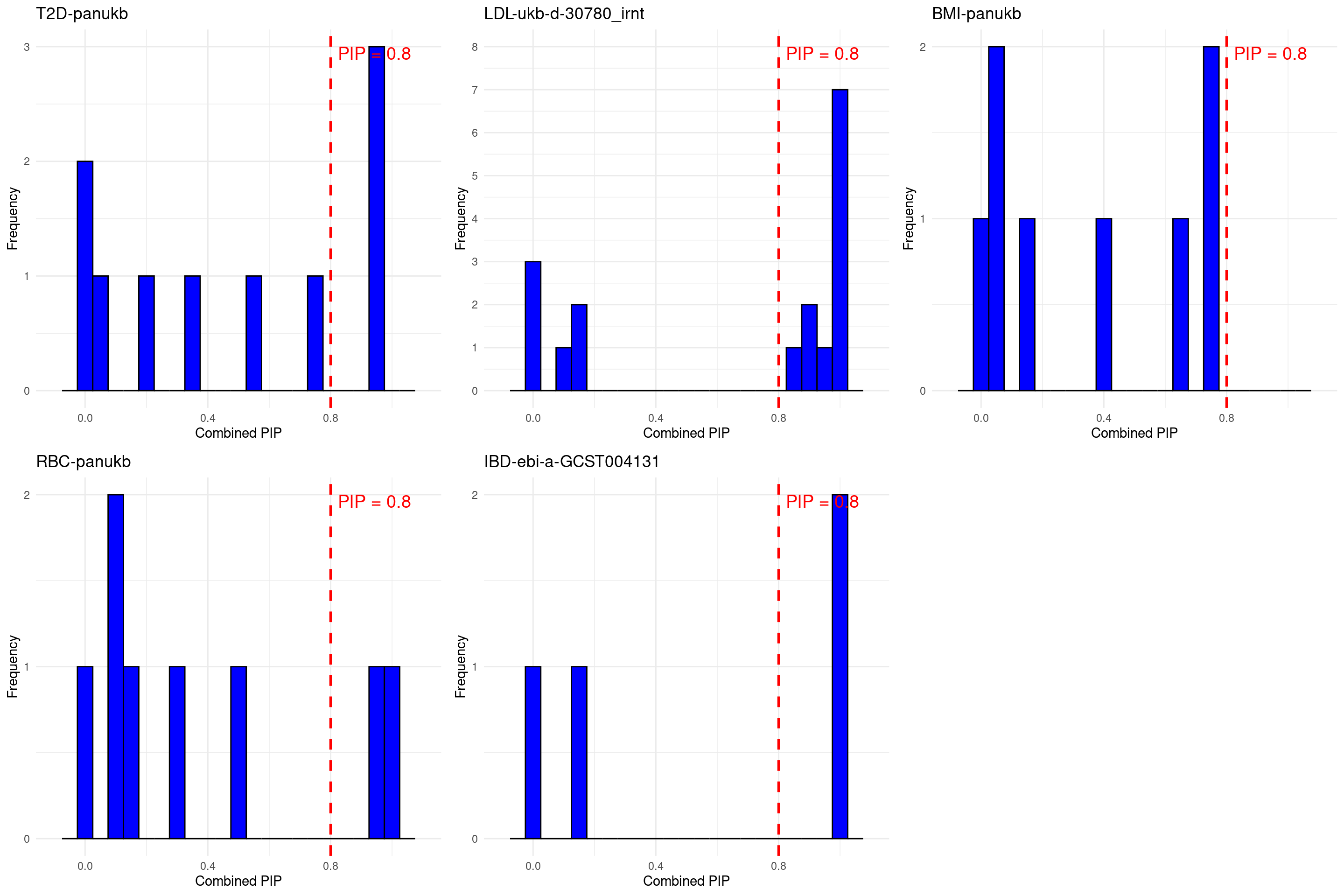
Silver standard for LDL – details
https://sq-96.github.io/multigroup_ctwas_analysis/LDL_silver_standard.html
Enrichment analysis – fractional model
Methods for enrichment analsis can be found here: https://sq-96.github.io/multigroup_ctwas_analysis/multi_group_6traits_15weights_ess_enrichment_genesymbol.html#Fractional_model
LDL-ukb-d-30780_irnt
Comparing multi-group and single-group results
trait <- "LDL-ukb-d-30780_irnt"
db <- "GO_Biological_Process_2023"
enrich_multi <- readRDS(paste0("/project/xinhe/xsun/multi_group_ctwas/13.post_processing_0103/results_downstream/enrich_fractional/enrichment_fractional_calibrated_blgeneset_summary_multigroup_", trait, "_", db, ".RDS"))
enrich_single <- readRDS(paste0("/project/xinhe/xsun/multi_group_ctwas/13.post_processing_0103/results_downstream/enrich_fractional/enrichment_fractional_calibrated_blgeneset_summary_singlegroup_", trait, "_", db, ".RDS"))
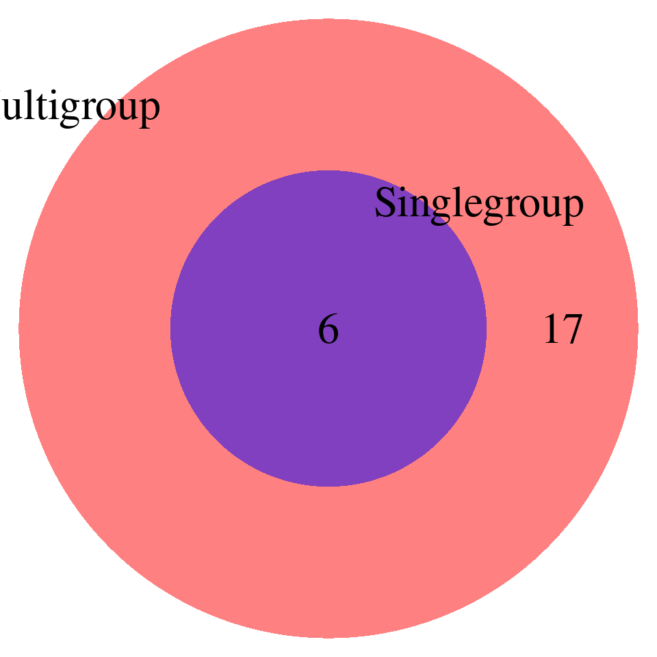
print("FDR_adjust < 0.05")[1] "FDR_adjust < 0.05"enrich_multi_sig <- enrich_multi[enrich_multi$fdr_calibrated < 0.05,]
enrich_single_sig <- enrich_multi[enrich_single$fdr_calibrated < 0.05,]
venn.plot <- draw.pairwise.venn(
area1 = nrow(enrich_multi_sig), # Size of Group A
area2 = nrow(enrich_single_sig), # Size of Group B
cross.area = sum(enrich_multi_sig$GO %in% enrich_single_sig$GO), # Overlap between Group A and Group B
category = c("Multigroup", "Singlegroup"), # Labels for the groups
fill = c("red", "blue"), # Colors for the groups
lty = "blank", # Line type for the circles
cex = 2, # Font size for the numbers
cat.cex = 2 # Font size for the labels
)
| Version | Author | Date |
|---|---|---|
| 25aaa64 | XSun | 2025-01-15 |
enrich_multi_unique <- enrich_multi_sig[!enrich_multi_sig$GO %in% enrich_single_sig$GO,]
enrich_multi_unique <- cbind(enrich_multi_unique$GO,enrich_multi_unique[,1:ncol(enrich_multi_unique)-1])
DT::datatable(enrich_multi_unique,caption = htmltools::tags$caption( style = 'caption-side: left; text-align: left; color:black;  font-size:150% ;','Enrichment results -- unique GO terms found by multi-group analysis'),options = list(pageLength = 10) )
# enrich_single_unique <- enrich_single_sig[!enrich_single_sig$GO %in% enrich_multi_sig$GO,]
# DT::datatable(enrich_single_unique,caption = htmltools::tags$caption( style = 'caption-side: left; text-align: left; color:black; font-size:150% ;','Enrichment results -- unique GO terms found by single-group analysis, FDR < 0.05'),options = list(pageLength = 10) )Notes from chatgpt
unique GO terms found by multi-group analysis:
- Strongest Direct Connections:
- Regulation of LDL particle clearance (GO:0010988).
- Negative regulation of lipoprotein clearance (GO:0010985).
- Endocytosis (GO:0006897).
- Sterol/cholesterol biosynthesis and transport (GO:0015918, GO:0016126, GO:0006695).
- Indirect Connections via Metabolic Regulation:
- Cellular response to insulin stimulus (GO:0032869).
- VLDL and triglyceride remodeling (GO:0034372, GO:0034370).
print("FDR_adjust < 0.1")[1] "FDR_adjust < 0.1"enrich_multi_sig <- enrich_multi[enrich_multi$fdr_calibrated < 0.1,]
enrich_single_sig <- enrich_multi[enrich_single$fdr_calibrated < 0.1,]
venn.plot <- draw.pairwise.venn(
area1 = nrow(enrich_multi_sig), # Size of Group A
area2 = nrow(enrich_single_sig), # Size of Group B
cross.area = sum(enrich_multi_sig$GO %in% enrich_single_sig$GO), # Overlap between Group A and Group B
category = c("Multigroup", "Singlegroup"), # Labels for the groups
fill = c("red", "blue"), # Colors for the groups
lty = "blank", # Line type for the circles
cex = 2, # Font size for the numbers
cat.cex = 2 # Font size for the labels
)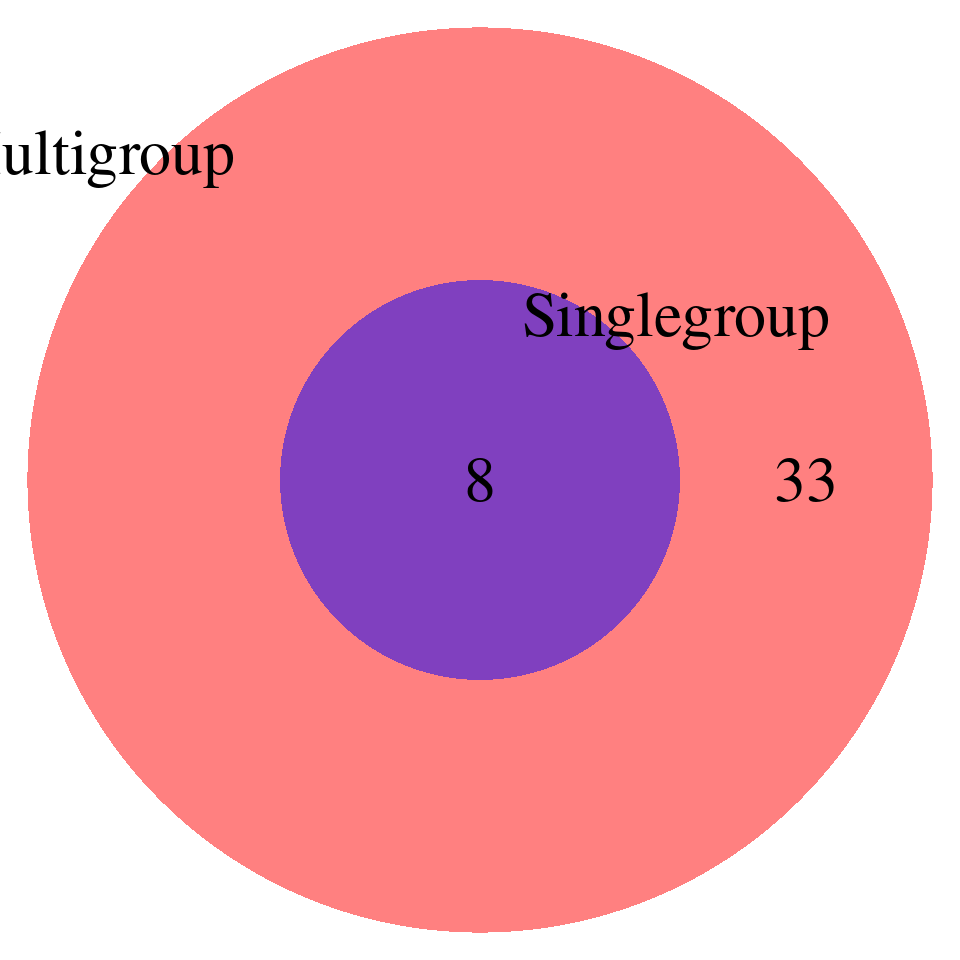
enrich_multi_unique <- enrich_multi_sig[!enrich_multi_sig$GO %in% enrich_single_sig$GO,]
enrich_multi_unique <- cbind(enrich_multi_unique$GO,enrich_multi_unique[,1:ncol(enrich_multi_unique)-1])

DT::datatable(enrich_multi_unique,caption = htmltools::tags$caption( style = 'caption-side: left; text-align: left; color:black;  font-size:150% ;','Enrichment results -- unique GO terms found by multi-group analysis'),options = list(pageLength = 10) )
# enrich_single_unique <- enrich_single_sig[!enrich_single_sig$GO %in% enrich_multi_sig$GO,]
# DT::datatable(enrich_single_unique,caption = htmltools::tags$caption( style = 'caption-side: left; text-align: left; color:black; font-size:150% ;','Enrichment results -- unique GO terms found by single-group analysis, FDR < 0.1'),options = list(pageLength = 10) )Additional signals from 16 additional GO terms at FDR < 0.1
Notes from chatgpt
- Directly Relevant GO Terms:
- Intestinal Cholesterol Absorption (GO:0030299).
- Intestinal Lipid Absorption (GO:0098856).
- Regulation of Cholesterol Transport (GO:0032374).
- High-Density Lipoprotein Particle Remodeling (GO:0034375).
- Regulation of Receptor Recycling (GO:0001919).
- Indirectly Relevant GO Terms:
- Sphingolipid and Phospholipid Biosynthetic Processes (GO:0030148, GO:0008654).
- Unsaturated Fatty Acid and Phosphatidic Acid Processes (GO:0033559, GO:0006654).
Comparing multi-group and magma
print("FDR_adjust < 0.05")[1] "FDR_adjust < 0.05"enrich_multi_sig <- enrich_multi[enrich_multi$fdr_calibrated < 0.05,]
enrich_single_sig <- enrich_multi[enrich_single$fdr_calibrated < 0.05,]
magma <- read.table(paste0("/project/xinhe/xsun/multi_group_ctwas/13.post_processing_0103/magma/",trait,"_",db,".gsa.out"),
header = TRUE, # The file has a header
sep = "", # Use whitespace as the separator
comment.char = "#", # Ignore lines starting with "#"
fill = TRUE, # Fill in missing values
quote = "", # Avoid issues with single quotes
check.names = FALSE) # Keep the original column names
magma$fdr <- p.adjust(as.numeric(magma$P),method = "fdr")
magma$FULL_NAME <- gsub("_", " ", magma$FULL_NAME)
magma_sig <- magma[magma$fdr < 0.05,]
venn.plot <- draw.pairwise.venn(
area1 = nrow(enrich_multi_sig), # Size of Group A
area2 = nrow(magma_sig), # Size of Group B
cross.area = sum(enrich_multi_sig$GO %in% magma_sig$FULL_NAME), # Overlap between Group A and Group B
category = c("Multigroup", "Magma"), # Labels for the groups
fill = c("red", "blue"), # Colors for the groups
lty = "blank", # Line type for the circles
cex = 2, # Font size for the numbers
cat.cex = 2 # Font size for the labels
)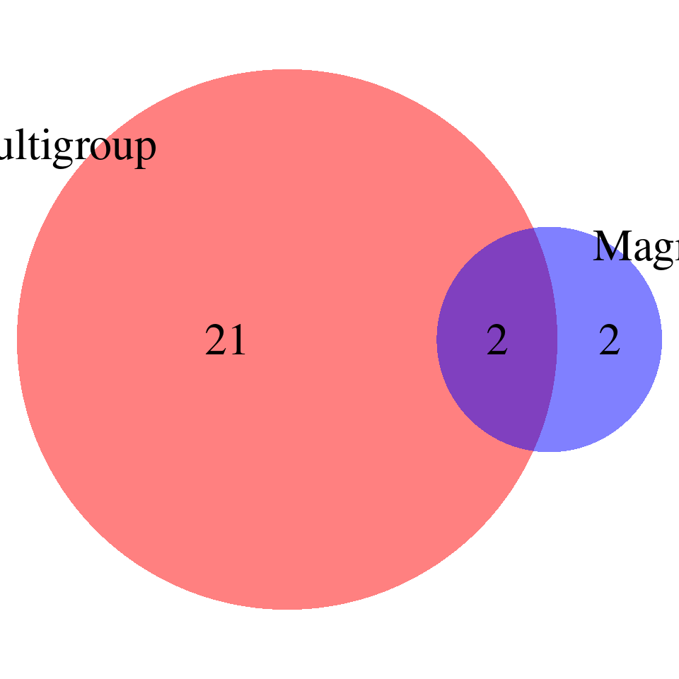
enrich_multi_unique <- enrich_multi_sig[!enrich_multi_sig$GO %in% magma_sig$FULL_NAME,]
enrich_multi_unique <- cbind(enrich_multi_unique$GO,enrich_multi_unique[,1:ncol(enrich_multi_unique)-1])

DT::datatable(enrich_multi_unique,caption = htmltools::tags$caption( style = 'caption-side: left; text-align: left; color:black;  font-size:150% ;','Enrichment results -- unique GO terms found by multi-group analysis'),options = list(pageLength = 10) )
magma_unique <- magma_sig[!magma_sig$FULL_NAME %in%enrich_multi_sig$GO,]
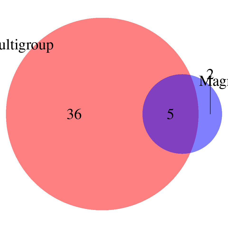
DT::datatable(magma_unique,caption = htmltools::tags$caption( style = 'caption-side: left; text-align: left; color:black; font-size:150% ;','Enrichment results -- unique GO terms found by MAGMA'),options = list(pageLength = 10) )print("FDR_adjust < 0.1")[1] "FDR_adjust < 0.1"enrich_multi_sig <- enrich_multi[enrich_multi$fdr_calibrated < 0.1,]
enrich_single_sig <- enrich_multi[enrich_single$fdr_calibrated < 0.1,]
magma <- read.table(paste0("/project/xinhe/xsun/multi_group_ctwas/13.post_processing_0103/magma/",trait,"_",db,".gsa.out"),
header = TRUE, # The file has a header
sep = "", # Use whitespace as the separator
comment.char = "#", # Ignore lines starting with "#"
fill = TRUE, # Fill in missing values
quote = "", # Avoid issues with single quotes
check.names = FALSE) # Keep the original column names
magma$fdr <- p.adjust(as.numeric(magma$P),method = "fdr")
magma$FULL_NAME <- gsub("_", " ", magma$FULL_NAME)
magma_sig <- magma[magma$fdr < 0.1,]
venn.plot <- draw.pairwise.venn(
area1 = nrow(enrich_multi_sig), # Size of Group A
area2 = nrow(magma_sig), # Size of Group B
cross.area = sum(enrich_multi_sig$GO %in% magma_sig$FULL_NAME), # Overlap between Group A and Group B
category = c("Multigroup", "Magma"), # Labels for the groups
fill = c("red", "blue"), # Colors for the groups
lty = "blank", # Line type for the circles
cex = 2, # Font size for the numbers
cat.cex = 2 # Font size for the labels
)
| Version | Author | Date |
|---|---|---|
| d47a369 | XSun | 2025-01-17 |
enrich_multi_unique <- enrich_multi_sig[!enrich_multi_sig$GO %in% magma_sig$FULL_NAME,]
enrich_multi_unique <- cbind(enrich_multi_unique$GO,enrich_multi_unique[,1:ncol(enrich_multi_unique)-1])

DT::datatable(enrich_multi_unique,caption = htmltools::tags$caption( style = 'caption-side: left; text-align: left; color:black;  font-size:150% ;','Enrichment results -- unique GO terms found by multi-group analysis'),options = list(pageLength = 10) )
magma_unique <- magma_sig[!magma_sig$FULL_NAME %in%enrich_multi_sig$GO,]
DT::datatable(magma_unique,caption = htmltools::tags$caption( style = 'caption-side: left; text-align: left; color:black; font-size:150% ;','Enrichment results -- unique GO terms found by MAGMA'),options = list(pageLength = 10) )Setting2: variance shared by all – pre-estimate L
Parameters
folder_results <- "/project/xinhe/shengqian/ctwas_GWAS_analysis/results_same_variance/"

all_var <-c()
for(trait in traits[!traits %in% brain_traits]){

  param <- readRDS(paste0(folder_results, "/", trait, "/", trait, ".param.RDS"))
  gwas_n <- samplesize[trait]

  ctwas_parameters <- summarize_param(param, gwas_n)

  var <- cbind(names(ctwas_parameters$group_prior_var),ctwas_parameters$group_prior_var)
  colnames(var) <- c(paste0(trait,"_tissues"), paste0(trait,"_variance"))

  all_var <- cbind(all_var, var)
}

rownames(all_var) <- seq(1:nrow(all_var))

DT::datatable(all_var,caption = htmltools::tags$caption( style = 'caption-side: left; text-align: left; color:black;  font-size:150% ;','Variance for each group, non-psychiatric traits'),options = list(pageLength = 20) )
all_var <-c()
for(trait in brain_traits){
param <- readRDS(paste0(folder_results, "/", trait, "/", trait, ".param.RDS"))
gwas_n <- samplesize[trait]
ctwas_parameters <- summarize_param(param, gwas_n)
var <- cbind(names(ctwas_parameters$group_prior_var),ctwas_parameters$group_prior_var)
colnames(var) <- c(paste0(trait,"_tissues"), paste0(trait,"_variance"))
all_var <- cbind(all_var, var)
}
rownames(all_var) <- seq(1:nrow(all_var))
DT::datatable(all_var,caption = htmltools::tags$caption( style = 'caption-side: left; text-align: left; color:black; font-size:150% ;','Variance for each group, psychiatric traits'),options = list(pageLength = 20) )Genetic architecture of complex traits
Bubble plot: h2g partition across tissues and omics
Tissue order is from: https://sq-96.github.io/multigroup_ctwas_analysis/GWAS_tissue_selection.html
folder_results <- "/project/xinhe/shengqian/ctwas_GWAS_analysis/results_same_variance/"

p <- list()
for(trait in traits[!traits %in% brain_traits]){

  param <- readRDS(paste0(folder_results, "/", trait, "/", trait, ".param.RDS"))
  gwas_n <- samplesize[trait]
  tissue_order <- tissues_alltraits[[trait]]
  p[[length(p)+1]] <- create_bubble_plot(trait = trait,param = param,gwas_n = gwas_n, tissue_order = tissue_order)

}

print("Non-psychiatric")
[1] "Non-psychiatric"grid.arrange(grobs = p, ncol = 3, nrow = 5)
folder_results <- "/project/xinhe/shengqian/ctwas_GWAS_analysis/results_same_variance/"

p <- list()
for(trait in brain_traits){

  param <- readRDS(paste0(folder_results, "/", trait, "/", trait, ".param.RDS"))
  gwas_n <- samplesize[trait]
  tissue_order <- tissues_alltraits[[trait]]
  p[[length(p)+1]] <- create_bubble_plot(trait = trait,param = param,gwas_n = gwas_n, tissue_order = tissue_order)

}

print("psychiatric")
[1] "psychiatric"grid.arrange(grobs = p, ncol = 3, nrow = 2)
Reduce FP findings
Silver standard for T2D LDL BMI RBC IBD
traits_used_in_silver <- c("T2D-panukb","LDL-ukb-d-30780_irnt","BMI-panukb","RBC-panukb","IBD-ebi-a-GCST004131")
traits_silver <- c("T2D","LDL","BMI","RBC","IBD")
top_tissues <- c("Pituitary","Liver","Cells_Cultured_fibroblasts","Skin_Not_Sun_Exposed_Suprapubic","Whole_Blood")
names(top_tissues) <- c("T2D-panukb","LDL-ukb-d-30780_irnt","BMI-panukb","RBC-panukb","IBD-ebi-a-GCST004131")

#folder_single_results <- "/project/xinhe/shengqian/single_tissue_screen/processed_weights/expression_weights/"
folder_multi_results <- "/project/xinhe/shengqian/ctwas_GWAS_analysis/results_same_variance/"

stats_all <- c()
stats_all_twas <- c()
p <- list()
for (i in 1:length(traits_used_in_silver)){
#for (i in c(2)){
  known <- readRDS(paste0("/project/xinhe/xsun/multi_group_ctwas/data/silverstandard/known_annotations_",traits_silver[i],".RDS"))
  bystander <- readRDS(paste0("/project/xinhe/xsun/multi_group_ctwas/data/silverstandard/bystanders_",traits_silver[i],".RDS"))

  # single group results

  # tissue <- top_tissues[traits_used_in_silver[i]]
  #
  # z_gene_single <-readRDS(paste0(folder_single_results,"/",traits_used_in_silver[i],"/",traits_used_in_silver[i],"_",tissue,".z_gene.RDS"))
  # z_gene_single <- z_gene_single %>%
  #                 mutate(molecular_id = sub("\\|.*", "", id)) %>%  # Extract ENSG ID from id
  #                 left_join(mapping_two %>% dplyr::select(molecular_id, gene_name), by = "molecular_id")
  # z_gene_single$p <- z2p(z_gene_single$z)
  # z_gene_single$fdr <- p.adjust(z_gene_single$p, method = "bonferroni")
  # z_gene_single_sig <- z_gene_single[z_gene_single$fdr < 0.05,]
  #
  #
  # combined_pip_single <-readRDS(paste0(folder_single_results,"/",traits_used_in_silver[i],"/",traits_used_in_silver[i],"_",tissue,".combined_pip_bygroup_final.RDS"))
  # combined_pip_sig_single <- combined_pip_single[combined_pip_single$combined_pip > 0.8,]
  #
  #
  # stats_single <- c(traits_used_in_silver[i],"single-group-ctwaspip0.8",nrow(combined_pip_sig_single),length(known), sum(unique(z_gene_single$gene_name) %in% known),sum(combined_pip_sig_single$gene_name %in% known),length(bystander),sum(unique(z_gene_single$gene_name) %in% bystander) ,sum(combined_pip_sig_single$gene_name %in% bystander))
  # stats_single_twas <- c(traits_used_in_silver[i],"single-group-twasbonf0.05",nrow(z_gene_single_sig),length(known),sum(z_gene_single_sig$gene_name %in% known),length(bystander),sum(z_gene_single_sig$gene_name %in% bystander))

  # multi

  z_gene_multi <- readRDS(paste0(folder_multi_results,"/",traits_used_in_silver[i],"/",traits_used_in_silver[i],".z_gene.RDS"))
  z_gene_multi <- z_gene_multi %>%
                  mutate(molecular_id = sub("\\|.*", "", id)) %>%  # Extract ENSG ID from id
                  left_join(mapping_two %>% dplyr::select(molecular_id, gene_name), by = "molecular_id")
  z_gene_multi$p <- z2p(z_gene_multi$z)
  z_gene_multi$fdr <- p.adjust(z_gene_multi$p, method = "bonferroni")
  z_gene_multi_sig <- z_gene_multi[z_gene_multi$fdr < 0.05,]

  combined_pip_multi <-readRDS(paste0(folder_multi_results,"/",traits_used_in_silver[i],"/",traits_used_in_silver[i],".combined_pip_bygroup_final.RDS"))
  combined_pip_sig_multi <- combined_pip_multi[combined_pip_multi$combined_pip > 0.8,]

  stats_multi <- c(traits_used_in_silver[i],"multi-group-ctwaspip0.8",nrow(combined_pip_sig_multi),length(known), sum(unique(z_gene_multi$gene_name) %in% known),sum(combined_pip_sig_multi$gene_name %in% known),length(bystander),sum(unique(z_gene_multi$gene_name) %in% bystander) ,sum(combined_pip_sig_multi$gene_name %in% bystander))
  #stats_multi_twas <- c(traits_used_in_silver[i],"multi-group-twasbonf0.05",nrow(z_gene_multi_sig),length(known),sum(z_gene_multi_sig$gene_name %in% known),length(bystander),sum(z_gene_multi_sig$gene_name %in% bystander))
  stats_multi_twas <- c(traits_used_in_silver[i],"multi-group-twasbonf0.05",length(unique(z_gene_multi_sig$gene_name)),length(known),sum(unique(z_gene_multi_sig$gene_name) %in% known),length(bystander),sum(unique(z_gene_multi_sig$gene_name) %in% bystander))

  #stats_trait <- rbind(stats_single, stats_multi)
  stats_trait <- stats_multi
  stats_trait_twas <- stats_multi_twas
  #stats_trait_twas <- rbind(stats_single_twas, stats_multi_twas)

  stats_all <- rbind(stats_all,stats_trait)
  stats_all_twas <- rbind(stats_all_twas,stats_trait_twas)

  known_pip <- combined_pip_multi[combined_pip_multi$gene_name %in% known,]

  p[[i]] <- ggplot(data = known_pip, aes(x = combined_pip)) +
  geom_histogram(binwidth = 0.05, color = "black", fill = "blue") +
  geom_vline(xintercept = 0.8, color = "red", linetype = "dashed", size = 1) +
  annotate(
    "text",
    x = 0.8,
    y = max(table(cut(known_pip$combined_pip, breaks = seq(0, 1, 0.05)))),
    label = "PIP = 0.8",
    color = "red", hjust = -0.1, vjust = 1, size = 5
  ) +
  labs(
    title = traits_used_in_silver[i],
    x = "Combined PIP",
    y = "Frequency"
  ) +
  xlim(-0.1, 1.1) +
  scale_y_continuous(
    breaks = function(x) seq(ceiling(min(x, na.rm = TRUE)), floor(max(x, na.rm = TRUE)))
  ) +  # Generate integer breaks dynamically
  theme_minimal()
}

colnames(stats_all) <- c("trait","analysis","num_gene_pip08","num_gene_known","num_gene_known_imputable","num_gene_known_pip08","num_gene_bystander","num_gene_bystander_imputable","num_gene_bystander_pip08")
rownames(stats_all) <- seq(1:nrow(stats_all))
stats_all <- as.data.frame(stats_all)

stats_all$TP_rate <- as.numeric(stats_all$num_gene_known_pip08) / (as.numeric(stats_all$num_gene_known_pip08) + as.numeric(stats_all$num_gene_bystander_pip08))

DT::datatable(stats_all,caption = htmltools::tags$caption( style = 'caption-side: left; text-align: left; color:black;  font-size:150% ;','Comparing cTWAS results with silver standard genes'),options = list(pageLength = 10) )
colnames(stats_all_twas) <- c("trait","analysis","num_gene_bonf0.05","num_gene_known","num_gene_known_bonf0.05","num_gene_bystander","num_gene_bystander_bonf0.05")
rownames(stats_all_twas) <- seq(1:nrow(stats_all_twas))
stats_all_twas <- as.data.frame(stats_all_twas)
stats_all_twas$TP_rate <- as.numeric(stats_all_twas$num_gene_known_bonf0.05) / (as.numeric(stats_all_twas$num_gene_known_bonf0.05) + as.numeric(stats_all_twas$num_gene_bystander_bonf0.05))
DT::datatable(stats_all_twas,caption = htmltools::tags$caption( style = 'caption-side: left; text-align: left; color:black; font-size:150% ;','Comparing TWAS results with silver standard genes'),options = list(pageLength = 10) )grid.arrange(grobs = p, ncol = 3)
For BMI, the bystander genes with PIP > 0.8 are : “ERI1” “MTMR9” “CCND3” “ZBTB7A” “KCNH3” . No one is related to BMI
Setting3: variance shared by all – L=5
The power of gene discovery
SCZ-ieu-b-5102
trait <- "SCZ-ieu-b-5102"

folder_results_multi <- "/project/xinhe/shengqian/ctwas_GWAS_analysis/results_same_variance_L5/"
folder_results_single <- "/project/xinhe/shengqian/single_tissue_screen/processed_weights_L5/expression_weights/"
tissue_single <- "Brain_Hippocampus"

combined_pip_by_group_multi <- readRDS(paste0(folder_results_multi,trait,"/",trait,".combined_pip_bygroup_final.RDS"))
combined_pip_by_group_single <- readRDS(paste0(folder_results_single,trait,"/",trait,"_",tissue_single,".combined_pip_bygroup_final.RDS"))

combined_pip_by_group_sig_multi <- combined_pip_by_group_multi[combined_pip_by_group_multi$combined_pip > 0.8,]
combined_pip_by_group_sig_single <- combined_pip_by_group_single[combined_pip_by_group_single$combined_pip > 0.8,]

overlap <- combined_pip_by_group_sig_multi[combined_pip_by_group_sig_multi$gene_name %in% combined_pip_by_group_sig_single$gene_name,]

sprintf("# of unique genes from multi-group analysis = %s", nrow(combined_pip_by_group_sig_multi))
[1] "# of unique genes from multi-group analysis = 35"sprintf("# of unique genes from single-group analysis = %s", nrow(combined_pip_by_group_sig_single))[1] "# of unique genes from single-group analysis = 17"sprintf("# of overlapped genes = %s", nrow(overlap))[1] "# of overlapped genes = 7"plot_heatmap_byomics(heatmap_data = combined_pip_by_group_sig_multi[!combined_pip_by_group_sig_multi$gene_name %in% combined_pip_by_group_sig_single$gene_name,], main = "PIP partition for unique genes with PIP > 0.8 from multi-group analysis")
plot_heatmap_byomics(heatmap_data = combined_pip_by_group_sig_multi[combined_pip_by_group_sig_multi$gene_name %in% combined_pip_by_group_sig_single$gene_name,], main = "PIP partition for overlapped genes ")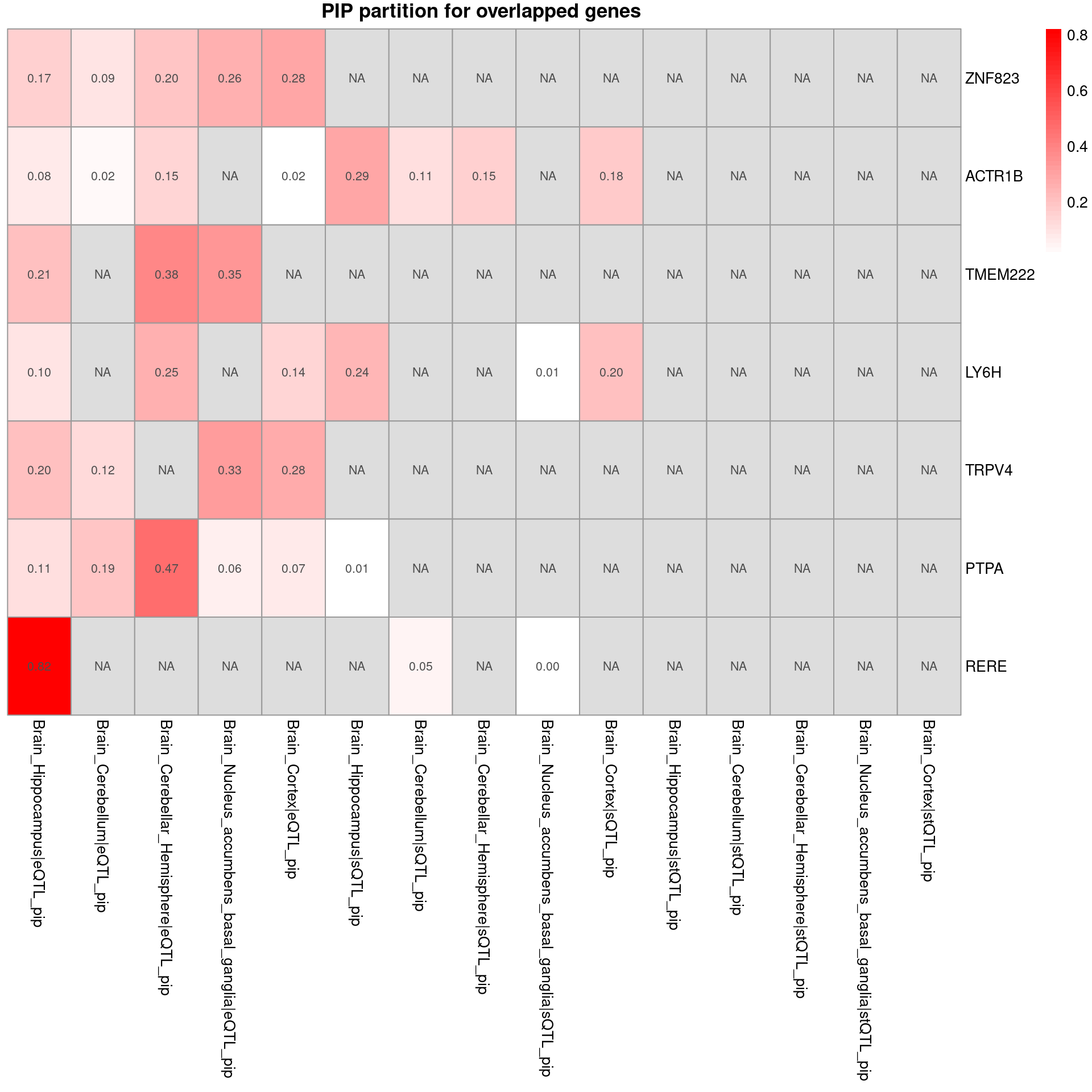
DT::datatable(combined_pip_by_group_sig_single[!combined_pip_by_group_sig_single$gene_name %in% combined_pip_by_group_sig_multi$gene_name,],caption = htmltools::tags$caption( style = 'caption-side: left; text-align: left; color:black; font-size:150% ;','Unique genes from single eqtl analysis'),options = list(pageLength = 10) )- Among the single eQTL unique genes, HIST1H2BN, HLA-DMB, and PPP1R16B may relate to SCZ
- Among the multi-group unique genes, NT5C2, DRD2, SDCCAG8 and ZKSCAN3 may relate to SCZ
- Among the overlapped genes, RERE, TMEM222 and TRPV4 may relate to SCZ
Reduce FP findings
Silver standard for T2D LDL BMI RBC IBD
traits_used_in_silver <- c("T2D-panukb","LDL-ukb-d-30780_irnt","BMI-panukb","RBC-panukb","IBD-ebi-a-GCST004131")
traits_silver <- c("T2D","LDL","BMI","RBC","IBD")
top_tissues <- c("Pituitary","Liver","Cells_Cultured_fibroblasts","Skin_Not_Sun_Exposed_Suprapubic","Whole_Blood")
names(top_tissues) <- c("T2D-panukb","LDL-ukb-d-30780_irnt","BMI-panukb","RBC-panukb","IBD-ebi-a-GCST004131")

folder_multi_results <- "/project/xinhe/shengqian/ctwas_GWAS_analysis/results_same_variance_L5/"

stats_all <- c()
stats_all_twas <- c()
p <- list()
for (i in 1:length(traits_used_in_silver)){
#for (i in c(2)){
  known <- readRDS(paste0("/project/xinhe/xsun/multi_group_ctwas/data/silverstandard/known_annotations_",traits_silver[i],".RDS"))
  bystander <- readRDS(paste0("/project/xinhe/xsun/multi_group_ctwas/data/silverstandard/bystanders_",traits_silver[i],".RDS"))

  # single group results

  # tissue <- top_tissues[traits_used_in_silver[i]]
  #
  # z_gene_single <-readRDS(paste0(folder_single_results,"/",traits_used_in_silver[i],"/",traits_used_in_silver[i],"_",tissue,".z_gene.RDS"))
  # z_gene_single <- z_gene_single %>%
  #                 mutate(molecular_id = sub("\\|.*", "", id)) %>%  # Extract ENSG ID from id
  #                 left_join(mapping_two %>% dplyr::select(molecular_id, gene_name), by = "molecular_id")
  # z_gene_single$p <- z2p(z_gene_single$z)
  # z_gene_single$fdr <- p.adjust(z_gene_single$p, method = "bonferroni")
  # z_gene_single_sig <- z_gene_single[z_gene_single$fdr < 0.05,]
  #
  #
  # combined_pip_single <-readRDS(paste0(folder_single_results,"/",traits_used_in_silver[i],"/",traits_used_in_silver[i],"_",tissue,".combined_pip_bygroup_final.RDS"))
  # combined_pip_sig_single <- combined_pip_single[combined_pip_single$combined_pip > 0.8,]
  #
  #
  # stats_single <- c(traits_used_in_silver[i],"single-group-ctwaspip0.8",nrow(combined_pip_sig_single),length(known), sum(unique(z_gene_single$gene_name) %in% known),sum(combined_pip_sig_single$gene_name %in% known),length(bystander),sum(unique(z_gene_single$gene_name) %in% bystander) ,sum(combined_pip_sig_single$gene_name %in% bystander))
  # stats_single_twas <- c(traits_used_in_silver[i],"single-group-twasbonf0.05",nrow(z_gene_single_sig),length(known),sum(z_gene_single_sig$gene_name %in% known),length(bystander),sum(z_gene_single_sig$gene_name %in% bystander))

  # multi

  z_gene_multi <- readRDS(paste0(folder_multi_results,"/",traits_used_in_silver[i],"/",traits_used_in_silver[i],".z_gene.RDS"))
  z_gene_multi <- z_gene_multi %>%
                  mutate(molecular_id = sub("\\|.*", "", id)) %>%  # Extract ENSG ID from id
                  left_join(mapping_two %>% dplyr::select(molecular_id, gene_name), by = "molecular_id")
  z_gene_multi$p <- z2p(z_gene_multi$z)
  z_gene_multi$fdr <- p.adjust(z_gene_multi$p, method = "bonferroni")
  z_gene_multi_sig <- z_gene_multi[z_gene_multi$fdr < 0.05,]

  combined_pip_multi <-readRDS(paste0(folder_multi_results,"/",traits_used_in_silver[i],"/",traits_used_in_silver[i],".combined_pip_bygroup_final.RDS"))
  combined_pip_sig_multi <- combined_pip_multi[combined_pip_multi$combined_pip > 0.8,]

  stats_multi <- c(traits_used_in_silver[i],"multi-group-ctwaspip0.8",nrow(combined_pip_sig_multi),length(known), sum(unique(z_gene_multi$gene_name) %in% known),sum(combined_pip_sig_multi$gene_name %in% known),length(bystander),sum(unique(z_gene_multi$gene_name) %in% bystander) ,sum(combined_pip_sig_multi$gene_name %in% bystander))
  #stats_multi_twas <- c(traits_used_in_silver[i],"multi-group-twasbonf0.05",nrow(z_gene_multi_sig),length(known),sum(z_gene_multi_sig$gene_name %in% known),length(bystander),sum(z_gene_multi_sig$gene_name %in% bystander))
  stats_multi_twas <- c(traits_used_in_silver[i],"multi-group-twasbonf0.05",length(unique(z_gene_multi_sig$gene_name)),length(known),sum(unique(z_gene_multi_sig$gene_name) %in% known),length(bystander),sum(unique(z_gene_multi_sig$gene_name) %in% bystander))

  #stats_trait <- rbind(stats_single, stats_multi)
  stats_trait <- stats_multi
  stats_trait_twas <- stats_multi_twas
  #stats_trait_twas <- rbind(stats_single_twas, stats_multi_twas)

  stats_all <- rbind(stats_all,stats_trait)
  stats_all_twas <- rbind(stats_all_twas,stats_trait_twas)

  known_pip <- combined_pip_multi[combined_pip_multi$gene_name %in% known,]

  p[[i]] <- ggplot(data = known_pip, aes(x = combined_pip)) +
  geom_histogram(binwidth = 0.05, color = "black", fill = "blue") +
  geom_vline(xintercept = 0.8, color = "red", linetype = "dashed", size = 1) +
  annotate(
    "text",
    x = 0.8,
    y = max(table(cut(known_pip$combined_pip, breaks = seq(0, 1, 0.05)))),
    label = "PIP = 0.8",
    color = "red", hjust = -0.1, vjust = 1, size = 5
  ) +
  labs(
    title = traits_used_in_silver[i],
    x = "Combined PIP",
    y = "Frequency"
  ) +
  xlim(-0.1, 1.1) +
  scale_y_continuous(
    breaks = function(x) seq(ceiling(min(x, na.rm = TRUE)), floor(max(x, na.rm = TRUE)))
  ) +  # Generate integer breaks dynamically
  theme_minimal()

}

colnames(stats_all) <- c("trait","analysis","num_gene_pip08","num_gene_known","num_gene_known_imputable","num_gene_known_pip08","num_gene_bystander","num_gene_bystander_imputable","num_gene_bystander_pip08")
rownames(stats_all) <- seq(1:nrow(stats_all))
stats_all <- as.data.frame(stats_all)

stats_all$TP_rate <- as.numeric(stats_all$num_gene_known_pip08) / (as.numeric(stats_all$num_gene_known_pip08) + as.numeric(stats_all$num_gene_bystander_pip08))

DT::datatable(stats_all,caption = htmltools::tags$caption( style = 'caption-side: left; text-align: left; color:black;  font-size:150% ;','Comparing cTWAS results with silver standard genes'),options = list(pageLength = 10) )
colnames(stats_all_twas) <- c("trait","analysis","num_gene_bonf0.05","num_gene_known","num_gene_known_bonf0.05","num_gene_bystander","num_gene_bystander_bonf0.05")
rownames(stats_all_twas) <- seq(1:nrow(stats_all_twas))
stats_all_twas <- as.data.frame(stats_all_twas)
stats_all_twas$TP_rate <- as.numeric(stats_all_twas$num_gene_known_bonf0.05) / (as.numeric(stats_all_twas$num_gene_known_bonf0.05) + as.numeric(stats_all_twas$num_gene_bystander_bonf0.05))
DT::datatable(stats_all_twas,caption = htmltools::tags$caption( style = 'caption-side: left; text-align: left; color:black; font-size:150% ;','Comparing TWAS results with silver standard genes'),options = list(pageLength = 10) )grid.arrange(grobs = p, ncol = 3)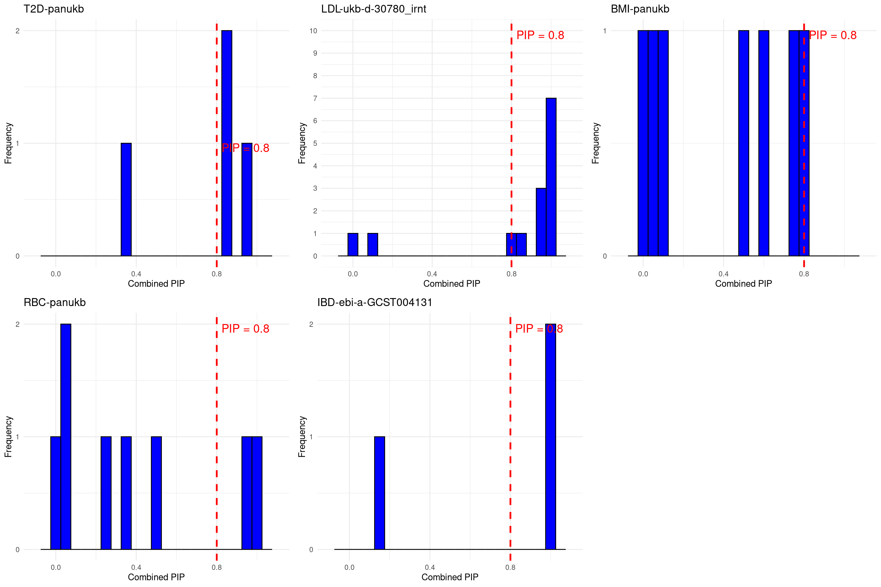
Bystander genes identified by cTWAS:
Notes from Perplexity
- T1D: “MAP2K7” “ZMIZ2”.
- LDL: “TRIM39” “SLC39A8” “NPC1L1” “CYP2A6” “HMGCR” “PRKD2” “CTSB” “ADH1B” “ACVR1C” “ABHD6” “SLC22A18” “MYPOP” “CCDC57” “GABBR1” “ADRB1” “APOC1” “DDX56” : NPC1L1 and HMGCR may relate to LDL
- BMI: “ADH1B” “NDUFA13” “TP53” “HLTF” “CASP7” “ETV5” “DMWD” “BAIAP2” “MTIF3” “YWHAQ” : ADH1B may relate to BMI
- RBC: “FDFT1” “CDC37L1” “COL4A3” “DUSP14” “OSER1” “ADH1B” : ADH1B may relate to RBC
- IBD: “LSP1”: may relate to IBD
sessionInfo()R version 4.2.0 (2022-04-22)
Platform: x86_64-pc-linux-gnu (64-bit)
Running under: CentOS Linux 7 (Core)
Matrix products: default
BLAS/LAPACK: /software/openblas-0.3.13-el7-x86_64/lib/libopenblas_haswellp-r0.3.13.so
locale:
[1] C
attached base packages:
[1] grid stats graphics grDevices utils datasets methods
[8] base
other attached packages:
[1] VennDiagram_1.7.3 futile.logger_1.4.3 pheatmap_1.0.12
[4] gridExtra_2.3 tidyr_1.3.0 dplyr_1.1.4
[7] ggplot2_3.5.1 ctwas_0.4.20.9001
loaded via a namespace (and not attached):
[1] colorspace_2.0-3 rjson_0.2.21
[3] ellipsis_0.3.2 rprojroot_2.0.3
[5] XVector_0.36.0 locuszoomr_0.2.1
[7] GenomicRanges_1.48.0 fs_1.5.2
[9] rstudioapi_0.13 farver_2.1.0
[11] DT_0.22 ggrepel_0.9.1
[13] bit64_4.0.5 AnnotationDbi_1.58.0
[15] fansi_1.0.3 xml2_1.3.3
[17] codetools_0.2-18 logging_0.10-108
[19] cachem_1.0.6 knitr_1.39
[21] jsonlite_1.8.0 workflowr_1.7.0
[23] Rsamtools_2.12.0 dbplyr_2.1.1
[25] png_0.1-7 readr_2.1.2
[27] compiler_4.2.0 httr_1.4.3
[29] assertthat_0.2.1 Matrix_1.5-3
[31] fastmap_1.1.0 lazyeval_0.2.2
[33] cli_3.6.1 formatR_1.12
[35] later_1.3.0 htmltools_0.5.2
[37] prettyunits_1.1.1 tools_4.2.0
[39] gtable_0.3.0 glue_1.6.2
[41] GenomeInfoDbData_1.2.8 rappdirs_0.3.3
[43] Rcpp_1.0.12 Biobase_2.56.0
[45] jquerylib_0.1.4 vctrs_0.6.5
[47] Biostrings_2.64.0 rtracklayer_1.56.0
[49] crosstalk_1.2.0 xfun_0.41
[51] stringr_1.5.1 lifecycle_1.0.4
[53] irlba_2.3.5 restfulr_0.0.14
[55] ensembldb_2.20.2 XML_3.99-0.14
[57] zlibbioc_1.42.0 zoo_1.8-10
[59] scales_1.3.0 gggrid_0.2-0
[61] hms_1.1.1 promises_1.2.0.1
[63] MatrixGenerics_1.8.0 ProtGenerics_1.28.0
[65] parallel_4.2.0 SummarizedExperiment_1.26.1
[67] lambda.r_1.2.4 RColorBrewer_1.1-3
[69] AnnotationFilter_1.20.0 LDlinkR_1.2.3
[71] yaml_2.3.5 curl_4.3.2
[73] memoise_2.0.1 sass_0.4.1
[75] biomaRt_2.54.1 stringi_1.7.6
[77] RSQLite_2.3.1 highr_0.9
[79] S4Vectors_0.34.0 BiocIO_1.6.0
[81] GenomicFeatures_1.48.3 BiocGenerics_0.42.0
[83] filelock_1.0.2 BiocParallel_1.30.3
[85] GenomeInfoDb_1.39.9 rlang_1.1.2
[87] pkgconfig_2.0.3 matrixStats_0.62.0
[89] bitops_1.0-7 evaluate_0.15
[91] lattice_0.20-45 purrr_1.0.2
[93] labeling_0.4.2 GenomicAlignments_1.32.0
[95] htmlwidgets_1.5.4 cowplot_1.1.1
[97] bit_4.0.4 tidyselect_1.2.0
[99] magrittr_2.0.3 R6_2.5.1
[101] IRanges_2.30.0 generics_0.1.2
[103] DelayedArray_0.22.0 DBI_1.2.2
[105] withr_2.5.0 pgenlibr_0.3.3
[107] pillar_1.9.0 whisker_0.4
[109] KEGGREST_1.36.3 RCurl_1.98-1.7
[111] mixsqp_0.3-43 tibble_3.2.1
[113] crayon_1.5.1 futile.options_1.0.1
[115] utf8_1.2.2 BiocFileCache_2.4.0
[117] plotly_4.10.0 tzdb_0.4.0
[119] rmarkdown_2.25 progress_1.2.2
[121] data.table_1.14.2 blob_1.2.3
[123] git2r_0.30.1 digest_0.6.29
[125] httpuv_1.6.5 stats4_4.2.0
[127] munsell_0.5.0 viridisLite_0.4.0
[129] bslib_0.3.1