Summary for multi-group analysis
XSun
2025-05-26
Last updated: 2025-05-26
Checks: 6 1
Knit directory: multigroup_ctwas_analysis/
This reproducible R Markdown analysis was created with workflowr (version 1.7.0). The Checks tab describes the reproducibility checks that were applied when the results were created. The Past versions tab lists the development history.
The R Markdown is untracked by Git. To know which version of the R
Markdown file created these results, you’ll want to first commit it to
the Git repo. If you’re still working on the analysis, you can ignore
this warning. When you’re finished, you can run
wflow_publish to commit the R Markdown file and build the
HTML.
Great job! The global environment was empty. Objects defined in the global environment can affect the analysis in your R Markdown file in unknown ways. For reproduciblity it’s best to always run the code in an empty environment.
The command set.seed(20231112) was run prior to running
the code in the R Markdown file. Setting a seed ensures that any results
that rely on randomness, e.g. subsampling or permutations, are
reproducible.
Great job! Recording the operating system, R version, and package versions is critical for reproducibility.
Nice! There were no cached chunks for this analysis, so you can be confident that you successfully produced the results during this run.
Great job! Using relative paths to the files within your workflowr project makes it easier to run your code on other machines.
Great! You are using Git for version control. Tracking code development and connecting the code version to the results is critical for reproducibility.
The results in this page were generated with repository version c791833. See the Past versions tab to see a history of the changes made to the R Markdown and HTML files.
Note that you need to be careful to ensure that all relevant files for
the analysis have been committed to Git prior to generating the results
(you can use wflow_publish or
wflow_git_commit). workflowr only checks the R Markdown
file, but you know if there are other scripts or data files that it
depends on. Below is the status of the Git repository when the results
were generated:
Ignored files:
    Ignored:    .Rhistory
    Ignored:    cv/

Untracked files:
    Untracked:  analysis/realdata_final_multigroup_summary.Rmd
    Untracked:  analysis/realdata_final_tissueselection_mingene0_summary.Rmd

Unstaged changes:
    Modified:   analysis/realdata_final_tissueselection_mingene0_exclude_brainprocessed.Rmd
    Modified:   analysis/realdata_final_tissueselection_mingene0_splicing_exclude_brainprocessed.Rmd
Note that any generated files, e.g. HTML, png, CSS, etc., are not included in this status report because it is ok for generated content to have uncommitted changes.
There are no past versions. Publish this analysis with
wflow_publish() to start tracking its development.
Introduction
This is a summary for tissues selected here: https://sq-96.github.io/multigroup_ctwas_analysis/realdata_final_tissueselection_mingene0_splicing_exclude_brainprocessed.html
library(ctwas)

source("/project/xinhe/xsun/multi_group_ctwas/functions/0.functions.R")
source("/project/xinhe/xsun/multi_group_ctwas/data/samplesize.R")

trait_nopsy <- c("LDL-ukb-d-30780_irnt","IBD-ebi-a-GCST004131","aFib-ebi-a-GCST006414","SBP-ukb-a-360",
                 "T1D-GCST90014023","T2D-panukb","ATH_gtexukb","BMI-panukb","HB-panukb",
                 "Height-panukb","HTN-panukb","PLT-panukb","RA-panukb","RBC-panukb",
                 "WBC-ieu-b-30")
trait_psy <- c("SCZ-ieu-b-5102","ASD-ieu-a-1185","BIP-ieu-b-5110","MDD-ieu-b-102","PD-ieu-b-7",
               "ADHD-ieu-a-1183","NS-ukb-a-230")
traits <- c(trait_nopsy,trait_psy)

colors <- c("#ff7f0e", "#2ca02c", "#d62728",  "#9467bd", "#8c564b", "#e377c2", "#7f7f7f",  "#bcbd22",  "#17becf",  "#f7b6d2",  "#c5b0d5",  "#9edae5", "#ffbb78",  "#98df8a",  "#ff9896" )


folder_results_single <- "/project/xinhe/xsun/multi_group_ctwas/22.singlegroup_0515/ctwas_output/expression/"
folder_results_multi <- "/project/xinhe/xsun/multi_group_ctwas/23.multi_group_0515/snakemake_outputs/"


generate_piecharts_for_trait <- function(title_top = NULL, colors = NULL) {

  if(is.null(colors)) {
    colors <- c("#ff7f0e", "#2ca02c", "#d62728",  "#9467bd", "#8c564b", "#e377c2", "#7f7f7f",  "#bcbd22",  "#17becf",  "#f7b6d2",  "#c5b0d5",  "#9edae5", "#ffbb78",  "#98df8a",  "#ff9896" )
  }

  pie_eqtl_single <- plot_piechart_single(ctwas_parameters_single, colors, by = "type", title = NULL)

  pie_eqtl_multi_type <- plot_piechart_topn(ctwas_parameters_multi, colors, by = "type", title = NULL)
  pie_eqtl_multi_context <- plot_piechart_topn(ctwas_parameters_multi, colors, by = "context", title = NULL, n_tissue = 10)

  # Function to fix panel size
  fix_panel_size <- function(plot, width = 2.1, height = 2) {
    set_panel_size(plot, width = unit(width, "in"), height = unit(height, "in"))
  }

  # Apply fixed panel size
  pie1 <- fix_panel_size(pie_eqtl_single)
  pie2 <- fix_panel_size(pie_eqtl_multi_type)
  pie3 <- fix_panel_size(pie_eqtl_multi_context)

  # Compute natural widths
  widths <- unit.c(grobWidth(pie1), grobWidth(pie2), grobWidth(pie3))

  # Arrange
  p <- grid.arrange(pie1, pie2, pie3,
                    ncol = 3,
                    widths = widths,
                    top = title_top)

  return(p)
}

# plot_overlap_barplot <- function(combined_pip_by_group_multi,
#                                  combined_pip_by_group_single,
#                                  PIP_cutoff = 0.8, tissue,
#                                  trait) {
#   # Filter genes by PIP cutoff
#   combined_pip_by_group_sig_multi <- combined_pip_by_group_multi[combined_pip_by_group_multi$combined_pip > PIP_cutoff, ]
#   combined_pip_by_group_sig_single <- combined_pip_by_group_single[combined_pip_by_group_single$combined_pip > PIP_cutoff, ]
#
#   # Extract gene names
#   multi_genes <- combined_pip_by_group_sig_multi$gene_name
#   single_genes <- combined_pip_by_group_sig_single$gene_name
#
#   # Compute overlap
#   overlap_genes <- intersect(multi_genes, single_genes)
#   single_genes_unique <- setdiff(single_genes,overlap_genes)
#   n_overlap <- length(overlap_genes)
#   n_multi <- length(multi_genes)
#   n_single <- length(single_genes)
#
#   # Construct data frame for plotting
#   df <- data.frame(
#     group = rep(c("Multi-group", paste0("Single-eQTL - \n", tissue)), each = 2),
#     part = rep(c("Overlap", "Unique"), 2),
#     count = c(n_overlap, n_multi - n_overlap, n_overlap, n_single - n_overlap)
#   )
#
#   # Ensure proper stacking order
#   df$part <- factor(df$part, levels = c("Unique", "Overlap"))
#
#   # Plot
#   p <- ggplot(df, aes(x = group, y = count, fill = part)) +
#     geom_bar(stat = "identity", width = 0.6) +
#     geom_text(aes(label = count), position = position_stack(vjust = 0.5), color = "white", size = 5) +
#     scale_fill_manual(values = c("Overlap" = "#1f77b4", "Unique" = "#ff7f0e")) +
#     labs(
#       x = "",
#       y = paste0("Number of Genes at PIP > ", PIP_cutoff),
#       title = trait,
#       fill = ""
#     ) +
#     theme_minimal(base_size = 14)
#
#   return(p,single_genes_unique)
# }

plot_overlap_barplot <- function(combined_pip_by_group_multi,
                                 combined_pip_by_group_single,
                                 PIP_cutoff = 0.8,
                                 tissue,
                                 trait,
                                 return_unique_genes = FALSE) {
  # Filter genes by PIP cutoff
  combined_pip_by_group_sig_multi <- combined_pip_by_group_multi[combined_pip_by_group_multi$combined_pip > PIP_cutoff, ]
  combined_pip_by_group_sig_single <- combined_pip_by_group_single[combined_pip_by_group_single$combined_pip > PIP_cutoff, ]

  # Extract gene names
  multi_genes <- combined_pip_by_group_sig_multi$gene_name
  single_genes <- combined_pip_by_group_sig_single$gene_name

  # Compute overlap
  overlap_genes <- intersect(multi_genes, single_genes)
  single_genes_unique <- setdiff(single_genes, overlap_genes)
  n_overlap <- length(overlap_genes)
  n_multi <- length(multi_genes)
  n_single <- length(single_genes)

  # Construct data frame for plotting
  df <- data.frame(
    group = rep(c("Multi-group", paste0("Single-eQTL - \n", tissue)), each = 2),
    part = rep(c("Overlap", "Unique"), 2),
    count = c(n_overlap, n_multi - n_overlap, n_overlap, n_single - n_overlap)
  )

  # Ensure proper stacking order
  df$part <- factor(df$part, levels = c("Unique", "Overlap"))

  # Plot
  p <- ggplot(df, aes(x = group, y = count, fill = part)) +
    geom_bar(stat = "identity", width = 0.6) +
    geom_text(aes(label = count), position = position_stack(vjust = 0.5), color = "white", size = 5) +
    scale_fill_manual(values = c("Overlap" = "#1f77b4", "Unique" = "#ff7f0e")) +
    labs(
      x = "",
      y = paste0("Number of Genes at PIP > ", PIP_cutoff),
      title = trait,
      fill = ""
    ) +
    theme_minimal(base_size = 14)

  if (return_unique_genes) {
    return(list(plot = p, single_genes_unique = single_genes_unique))
  } else {
    return(p)
  }
}


get_top_tissue <- function(group_pve) {
  # Remove QTL type to extract tissue names
  group_pve <- group_pve[-which(names(group_pve) =="SNP")]

  tissue_names <- sub("\\|.*", "", names(group_pve))

  # Sum PVE values across tissues
  tissue_pve <- tapply(group_pve, tissue_names, sum)

  # Return the tissue name with the highest total PVE
  top_tissue <- names(which.max(tissue_pve))
  return(top_tissue)
}
for (trait in traits){
cat("\n")
cat(trait)
cat("\n")
## parameters
gwas_n <- samplesize[trait]
param_multi <- readRDS(paste0(folder_results_multi,trait,"/",trait,".4qtls.thin1.shared_all.param.RDS"))
ctwas_parameters_multi <- summarize_param(param = param_multi,gwas_n = gwas_n)
top_tissue <- get_top_tissue(ctwas_parameters_multi$group_pve)
param_single <- readRDS(paste0(folder_results_single, trait, "/", trait, "_", top_tissue, ".thin1.shared_all.param.RDS"))
ctwas_parameters_single <- summarize_param(param_single, gwas_n)
title <- paste0(trait, ", top tissue: ", top_tissue)
grid.newpage()
print(generate_piecharts_for_trait(title_top = title))
## Overlap
PIP_cutoff <- 0.8
combined_pip_by_group_single <- readRDS(paste0(folder_results_single, trait, "/", trait, "_", top_tissue, ".combined_pip_bygroup_final.RDS"))
combined_pip_by_group_multi <- readRDS(paste0(folder_results_multi,trait,"/",trait,".4qtls.combined_pip_bygroup_final.RDS"))
grid.newpage()
print(plot_overlap_barplot(combined_pip_by_group_multi = combined_pip_by_group_multi, combined_pip_by_group_single = combined_pip_by_group_single,PIP_cutoff = PIP_cutoff,tissue = top_tissue,trait = trait,return_unique_genes = T))
## heatmaps
combined_pip_by_group_multi_sig <- combined_pip_by_group_multi[combined_pip_by_group_multi$combined_pip > PIP_cutoff,]
combined_pip_by_group_single_sig <- combined_pip_by_group_single[combined_pip_by_group_single$combined_pip > PIP_cutoff,]
combined_pip_by_group_multi_unique <- combined_pip_by_group_multi_sig[!combined_pip_by_group_multi_sig$gene_name %in% combined_pip_by_group_single_sig$gene_name, ]
grid.newpage()
if(nrow(combined_pip_by_group_multi_unique) > 0) {
print(plot_heatmap(heatmap_data = combined_pip_by_group_multi_unique, main = paste0("New genes identified by multigroup analysis, PIP>",PIP_cutoff),showPIP = T))
}
print(paste0("Unique genes from multigroup: ", paste0(combined_pip_by_group_multi_unique$gene_name, collapse = ", ")))
}
LDL-ukb-d-30780_irnt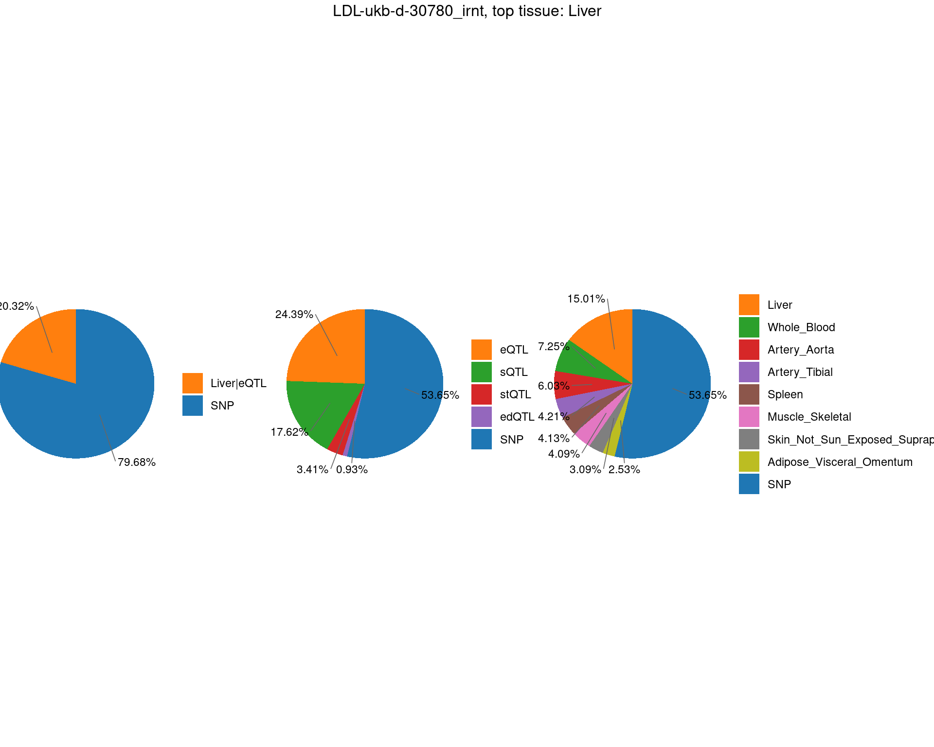
TableGrob (2 x 3) "arrange": 4 grobs
  z     cells    name                grob
1 1 (2-2,1-1) arrange      gtable[layout]
2 2 (2-2,2-2) arrange      gtable[layout]
3 3 (2-2,3-3) arrange      gtable[layout]
4 4 (1-1,1-3) arrange text[GRID.text.161]
$plot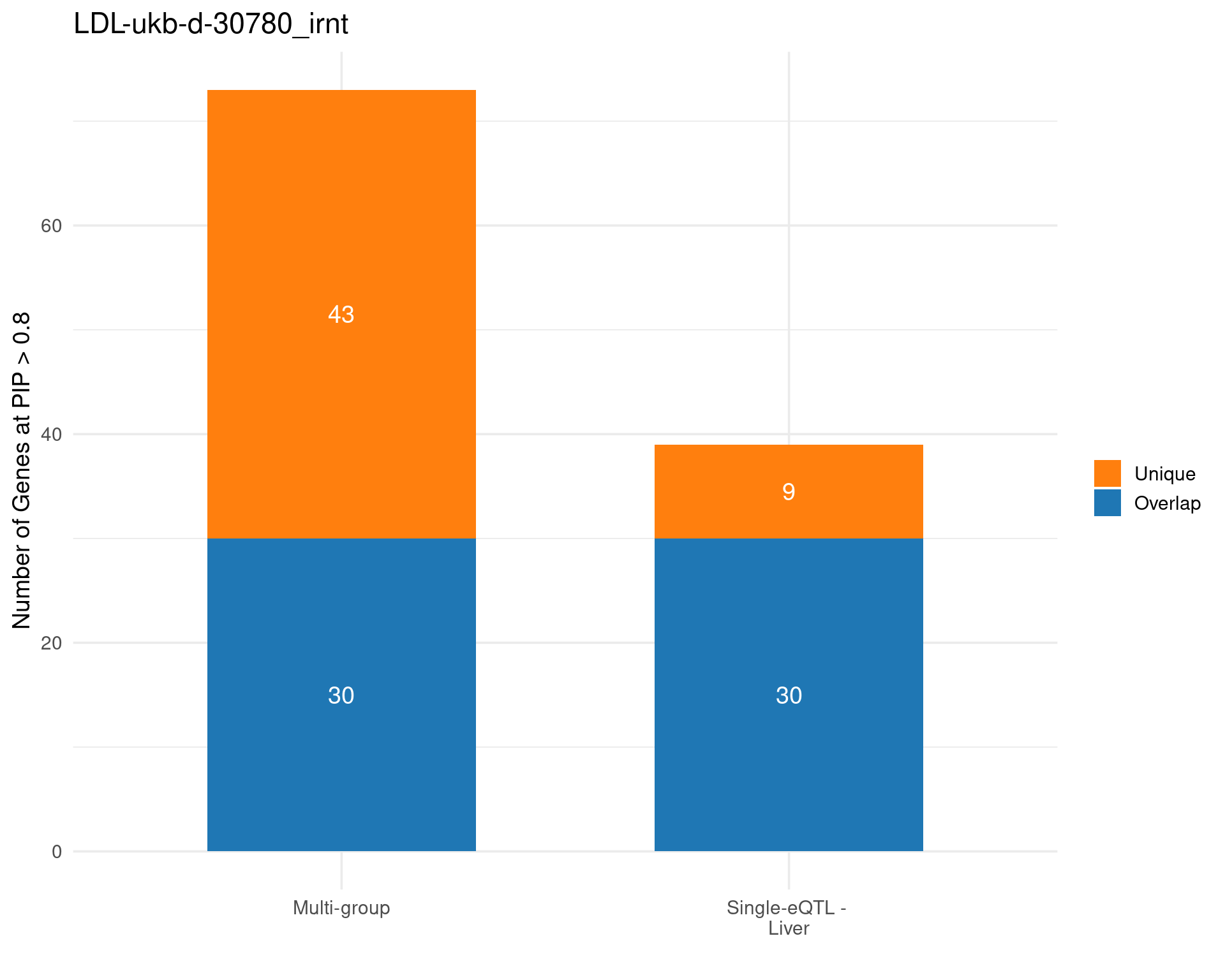
$single_genes_unique
[1] "PARP9"   "DDX56"   "ASAP3"   "MZF1"    "CLDN23"  "FUT2"    "VIL1"
[8] "KLHDC7A" "WBP1L" 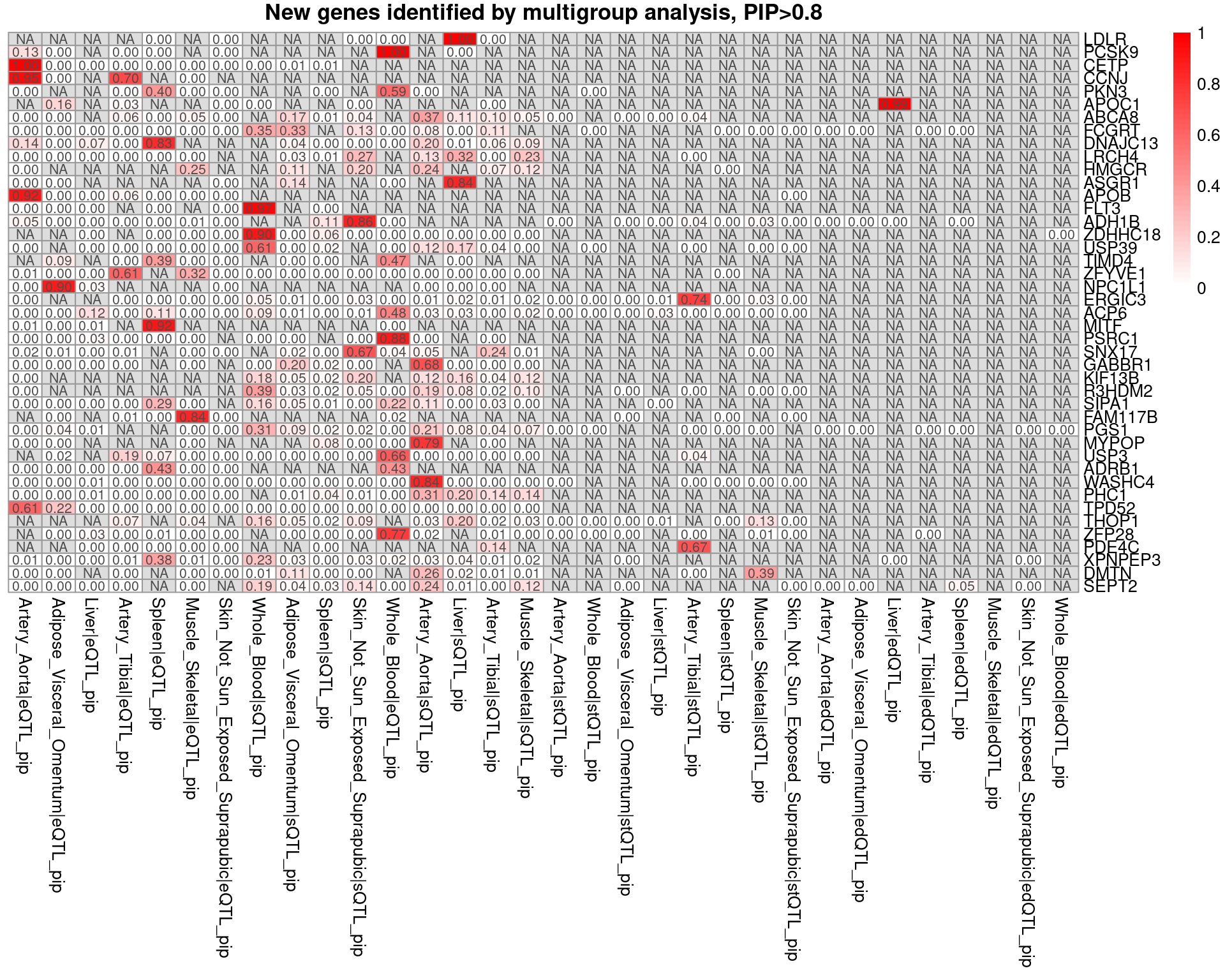
[1] "Unique genes from multigroup: LDLR, PCSK9, CETP, CCNJ, PKN3, APOC1, ABCA8, FCGRT, DNAJC13, LRCH4, HMGCR, ASGR1, APOB, FLT3, ADH1B, ZDHHC18, USP39, TIMD4, ZFYVE1, NPC1L1, ERGIC3, ACP6, MITF, PSRC1, SNX17, GABBR1, KIF13B, R3HDM2, SIPA1, FAM117B, PGS1, MYPOP, USP3, ADRB1, WASHC4, PHC1, TPD52, THOP1, ZFP28, PDE4C, XPNPEP3, DMTN, SEPT2"

IBD-ebi-a-GCST004131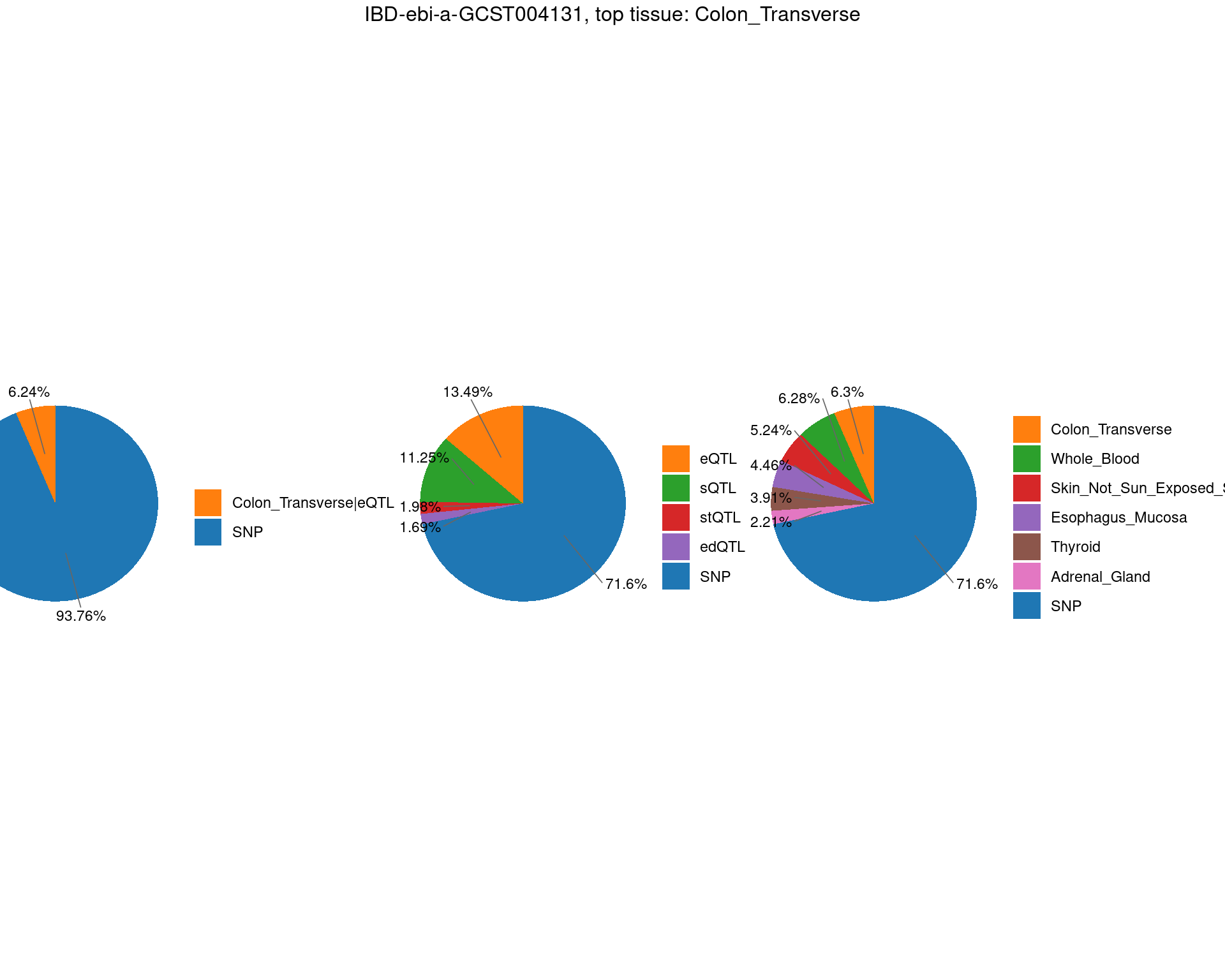
TableGrob (2 x 3) "arrange": 4 grobs
  z     cells    name                grob
1 1 (2-2,1-1) arrange      gtable[layout]
2 2 (2-2,2-2) arrange      gtable[layout]
3 3 (2-2,3-3) arrange      gtable[layout]
4 4 (1-1,1-3) arrange text[GRID.text.381]
$plot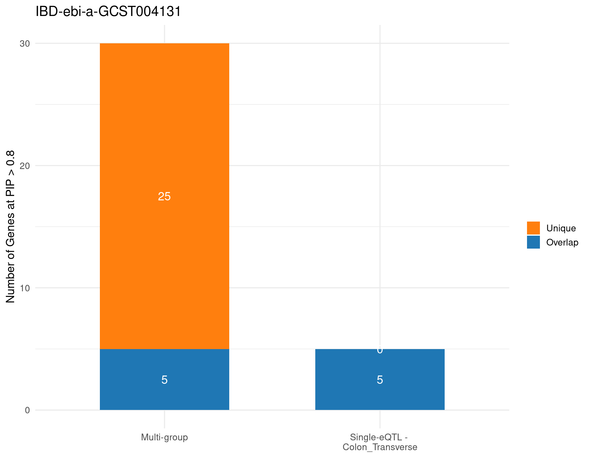
$single_genes_unique
character(0)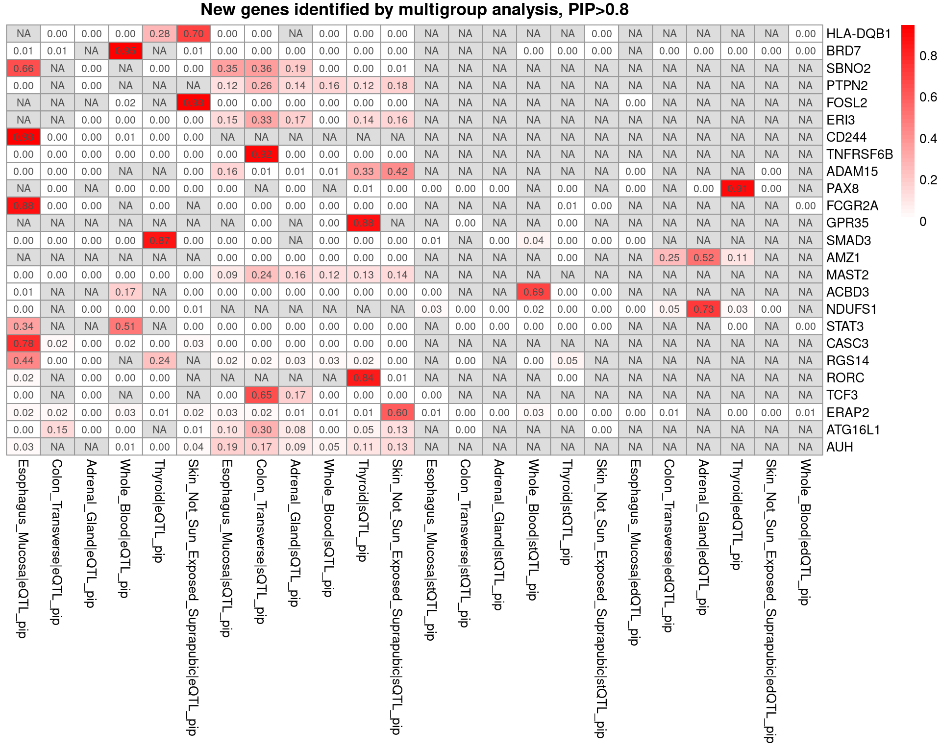
[1] "Unique genes from multigroup: HLA-DQB1, BRD7, SBNO2, PTPN2, FOSL2, ERI3, CD244, TNFRSF6B, ADAM15, PAX8, FCGR2A, GPR35, SMAD3, AMZ1, MAST2, ACBD3, NDUFS1, STAT3, CASC3, RGS14, RORC, TCF3, ERAP2, ATG16L1, AUH"

aFib-ebi-a-GCST006414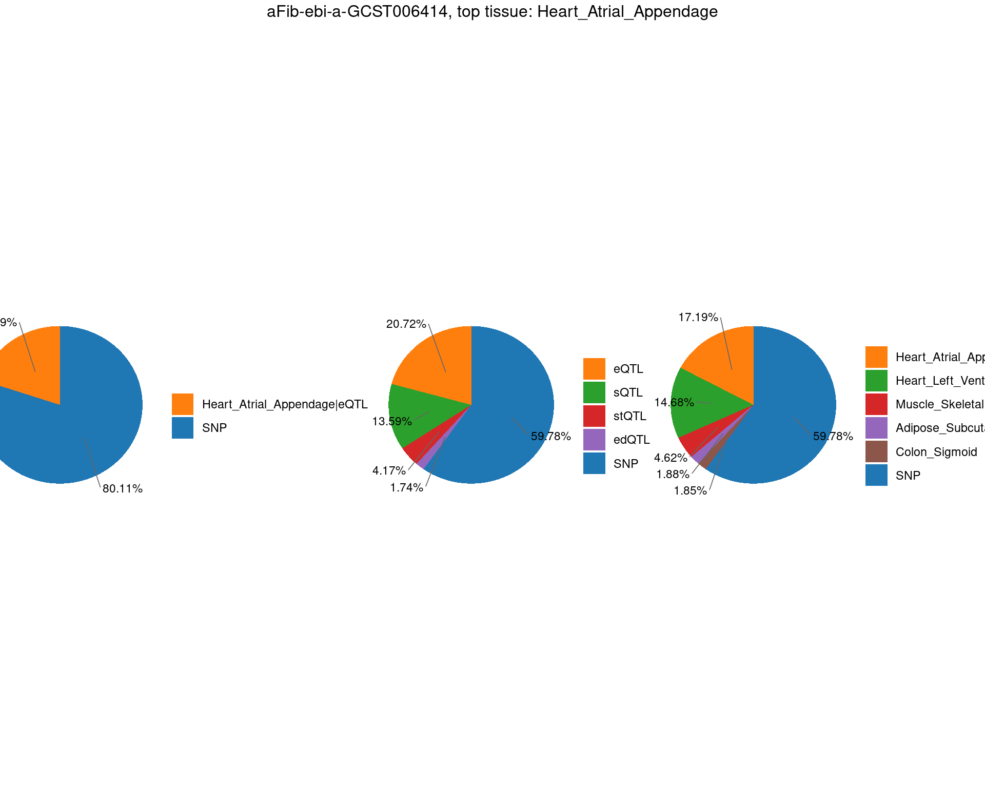
TableGrob (2 x 3) "arrange": 4 grobs
  z     cells    name                grob
1 1 (2-2,1-1) arrange      gtable[layout]
2 2 (2-2,2-2) arrange      gtable[layout]
3 3 (2-2,3-3) arrange      gtable[layout]
4 4 (1-1,1-3) arrange text[GRID.text.592]
$plot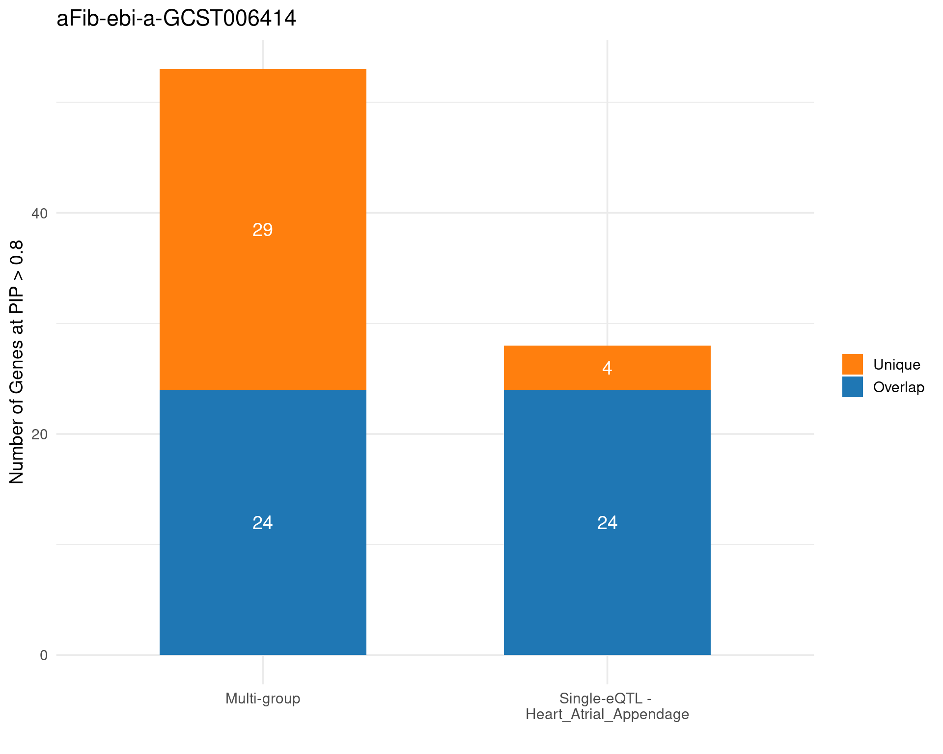
$single_genes_unique
[1] "DLEU1"   "DEK"     "MTSS1"   "C5orf47"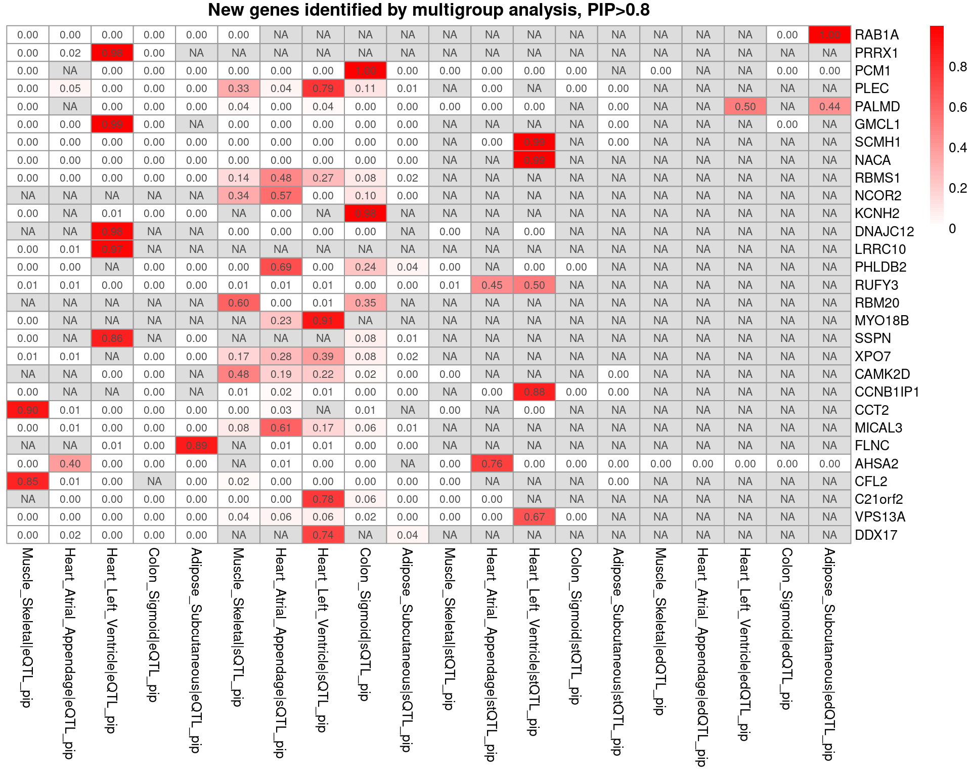
[1] "Unique genes from multigroup: RAB1A, PRRX1, PCM1, PLEC, PALMD, GMCL1, SCMH1, NACA, RBMS1, NCOR2, KCNH2, DNAJC12, LRRC10, PHLDB2, RUFY3, RBM20, MYO18B, SSPN, XPO7, CAMK2D, CCNB1IP1, CCT2, MICAL3, FLNC, AHSA2, CFL2, C21orf2, VPS13A, DDX17"

SBP-ukb-a-360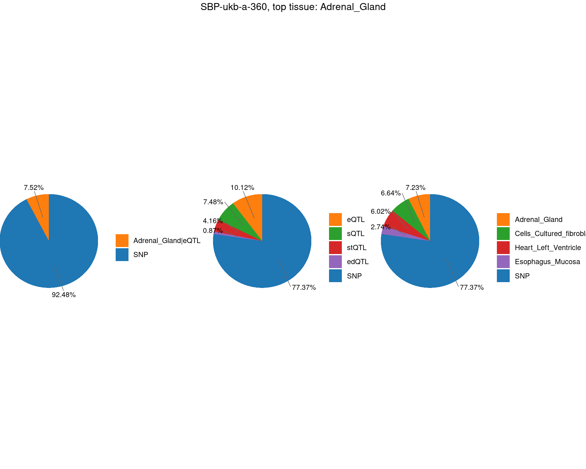
TableGrob (2 x 3) "arrange": 4 grobs
  z     cells    name                grob
1 1 (2-2,1-1) arrange      gtable[layout]
2 2 (2-2,2-2) arrange      gtable[layout]
3 3 (2-2,3-3) arrange      gtable[layout]
4 4 (1-1,1-3) arrange text[GRID.text.798]
$plot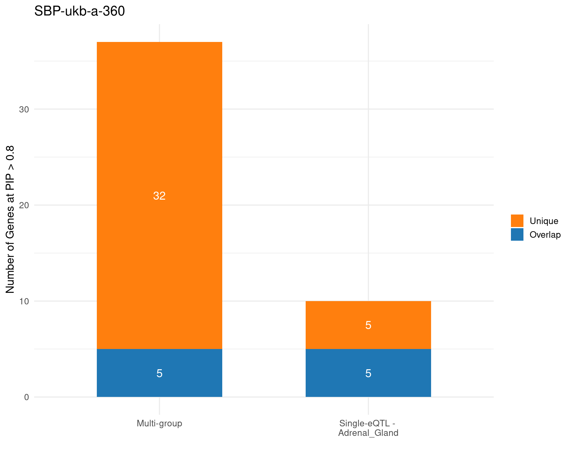
$single_genes_unique
[1] "ZNF467" "HFE" "SHISA8" "SHBG" "PLK2" 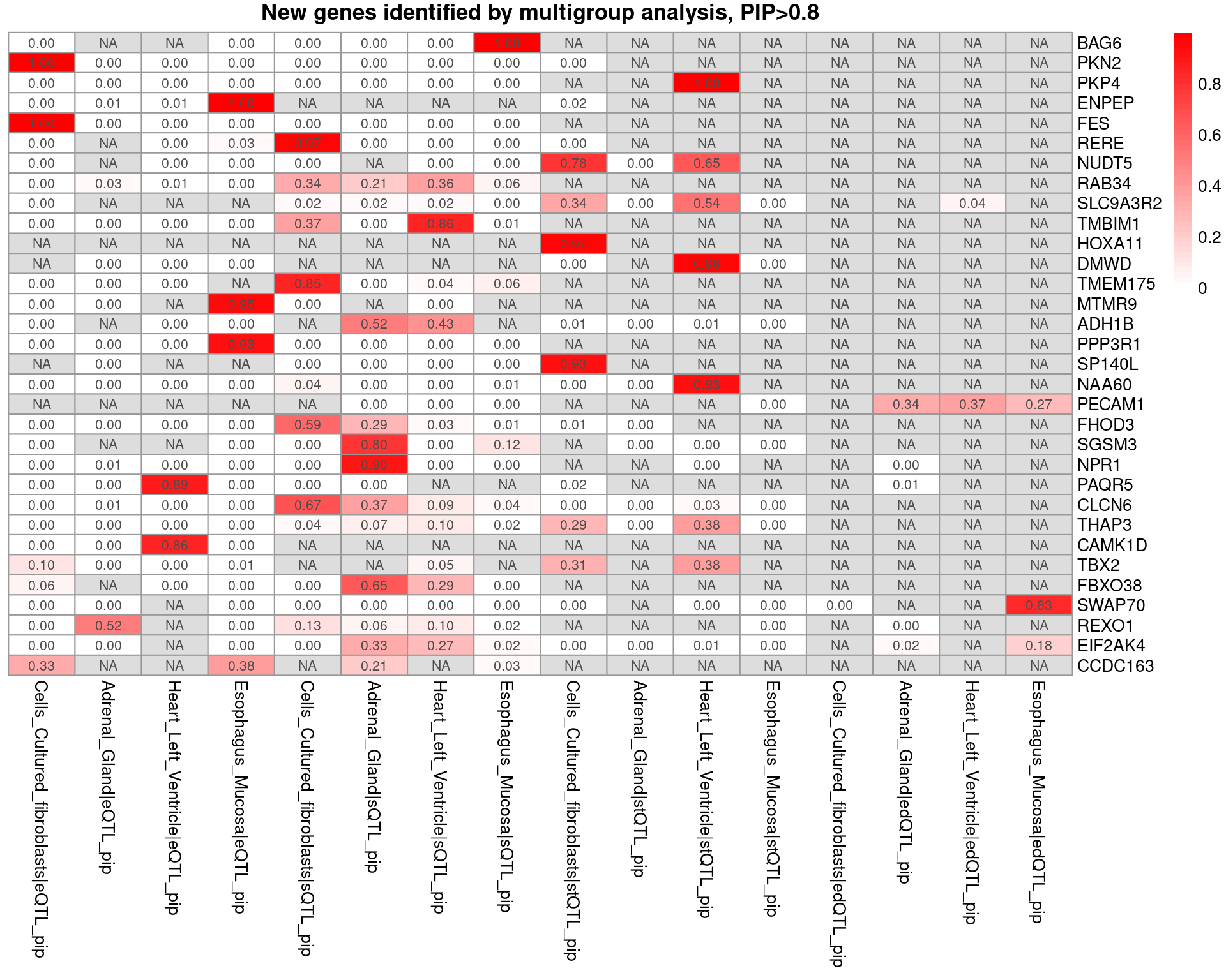
[1] "Unique genes from multigroup: BAG6, PKN2, PKP4, ENPEP, FES, RERE, NUDT5, RAB34, SLC9A3R2, TMBIM1, HOXA11, DMWD, TMEM175, MTMR9, ADH1B, PPP3R1, SP140L, NAA60, PECAM1, FHOD3, SGSM3, NPR1, PAQR5, CLCN6, THAP3, CAMK1D, TBX2, FBXO38, SWAP70, REXO1, EIF2AK4, CCDC163"

T1D-GCST90014023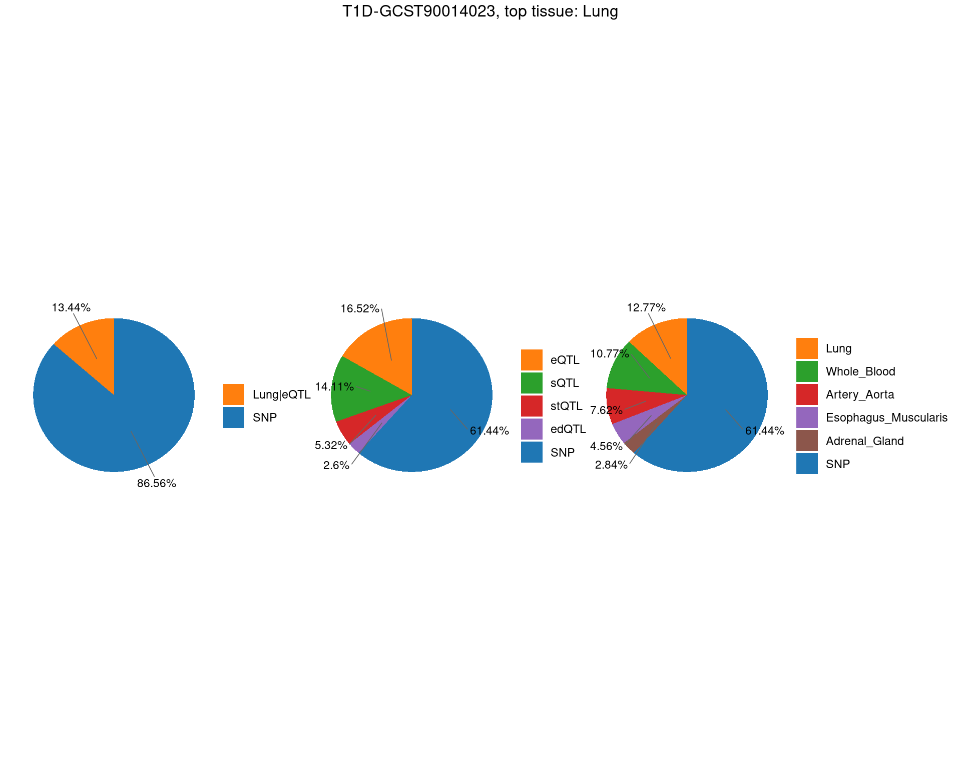
TableGrob (2 x 3) "arrange": 4 grobs
  z     cells    name                 grob
1 1 (2-2,1-1) arrange       gtable[layout]
2 2 (2-2,2-2) arrange       gtable[layout]
3 3 (2-2,3-3) arrange       gtable[layout]
4 4 (1-1,1-3) arrange text[GRID.text.1007]
$plot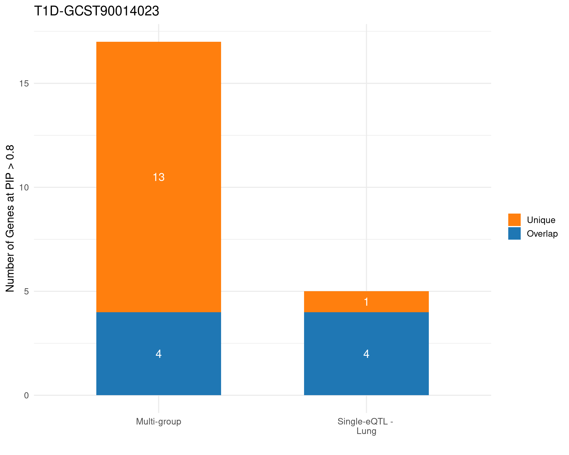
$single_genes_unique
[1] "ELMO3"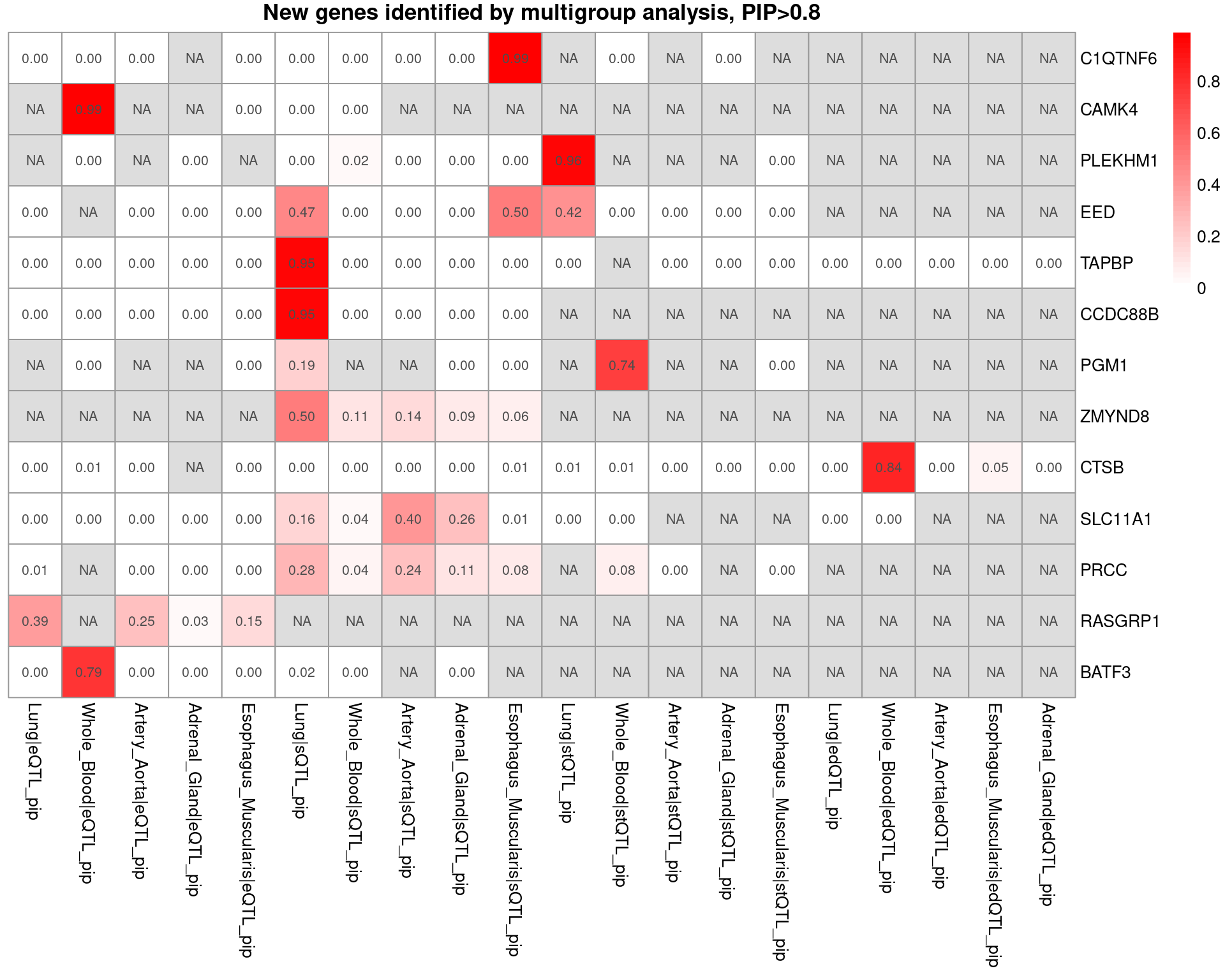
[1] "Unique genes from multigroup: C1QTNF6, CAMK4, PLEKHM1, EED, TAPBP, CCDC88B, PGM1, ZMYND8, CTSB, SLC11A1, PRCC, RASGRP1, BATF3"

T2D-panukb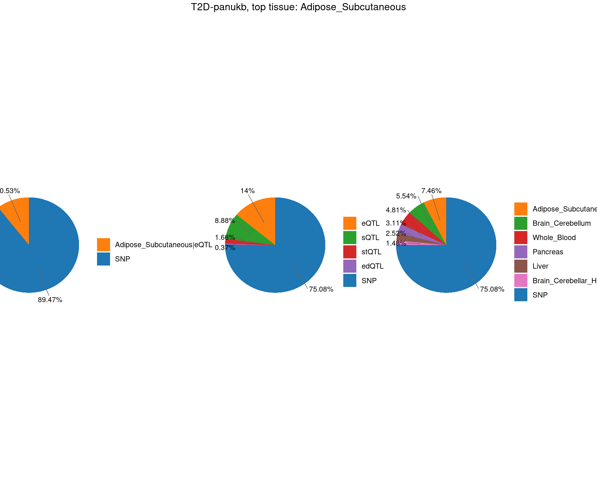
TableGrob (2 x 3) "arrange": 4 grobs
  z     cells    name                 grob
1 1 (2-2,1-1) arrange       gtable[layout]
2 2 (2-2,2-2) arrange       gtable[layout]
3 3 (2-2,3-3) arrange       gtable[layout]
4 4 (1-1,1-3) arrange text[GRID.text.1221]
$plot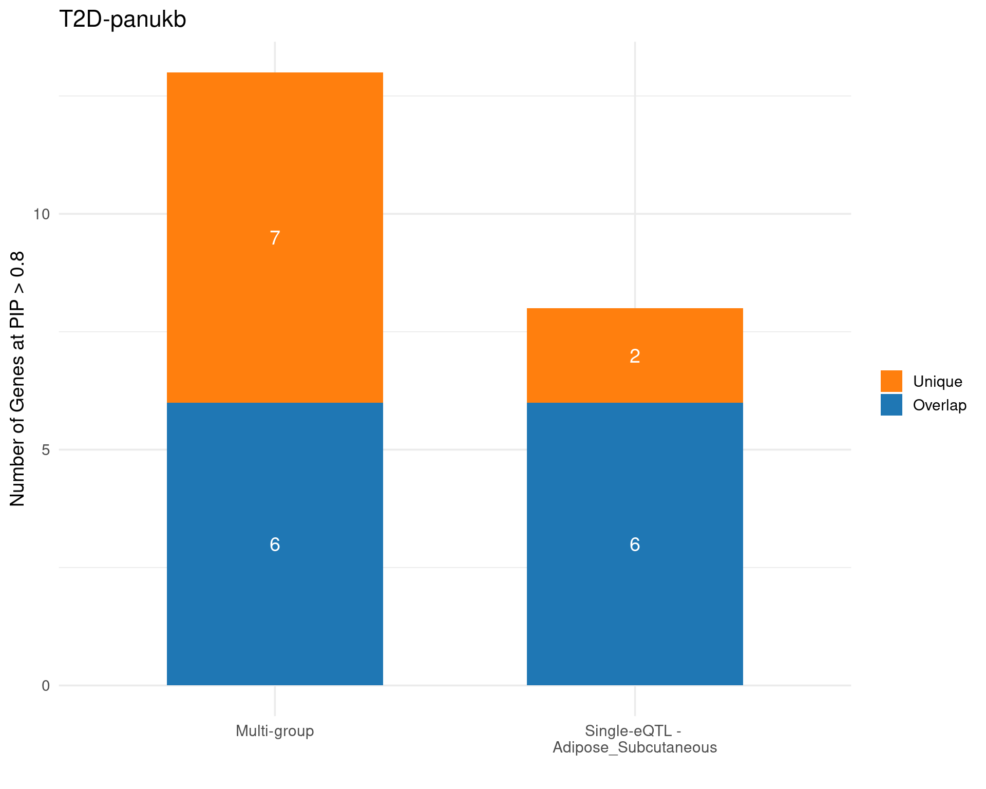
$single_genes_unique
[1] "CDKN1C" "JAZF1" 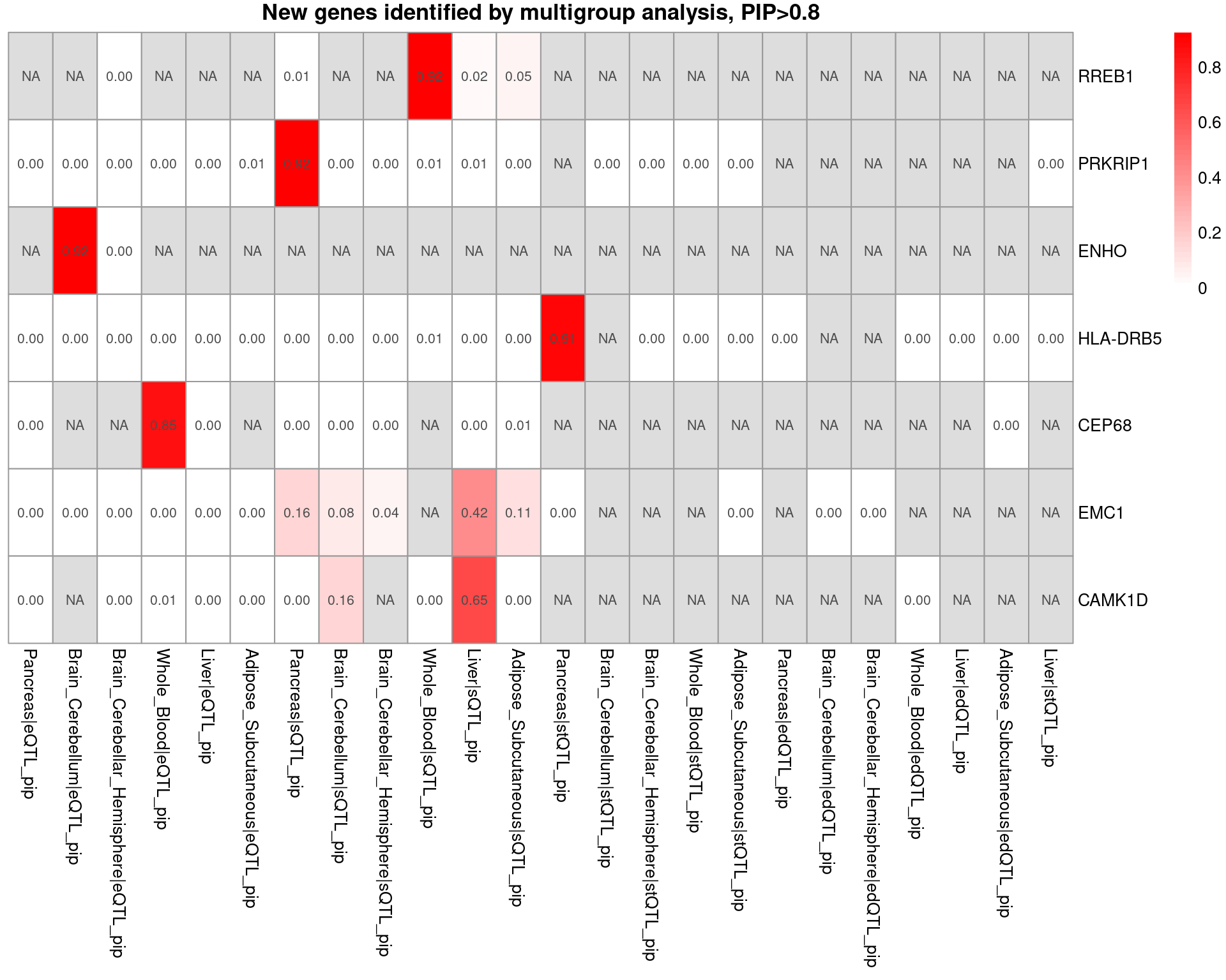
[1] "Unique genes from multigroup: RREB1, PRKRIP1, ENHO, HLA-DRB5, CEP68, EMC1, CAMK1D"

ATH_gtexukb
TableGrob (2 x 3) "arrange": 4 grobs
  z     cells    name                 grob
1 1 (2-2,1-1) arrange       gtable[layout]
2 2 (2-2,2-2) arrange       gtable[layout]
3 3 (2-2,3-3) arrange       gtable[layout]
4 4 (1-1,1-3) arrange text[GRID.text.1436]
$plot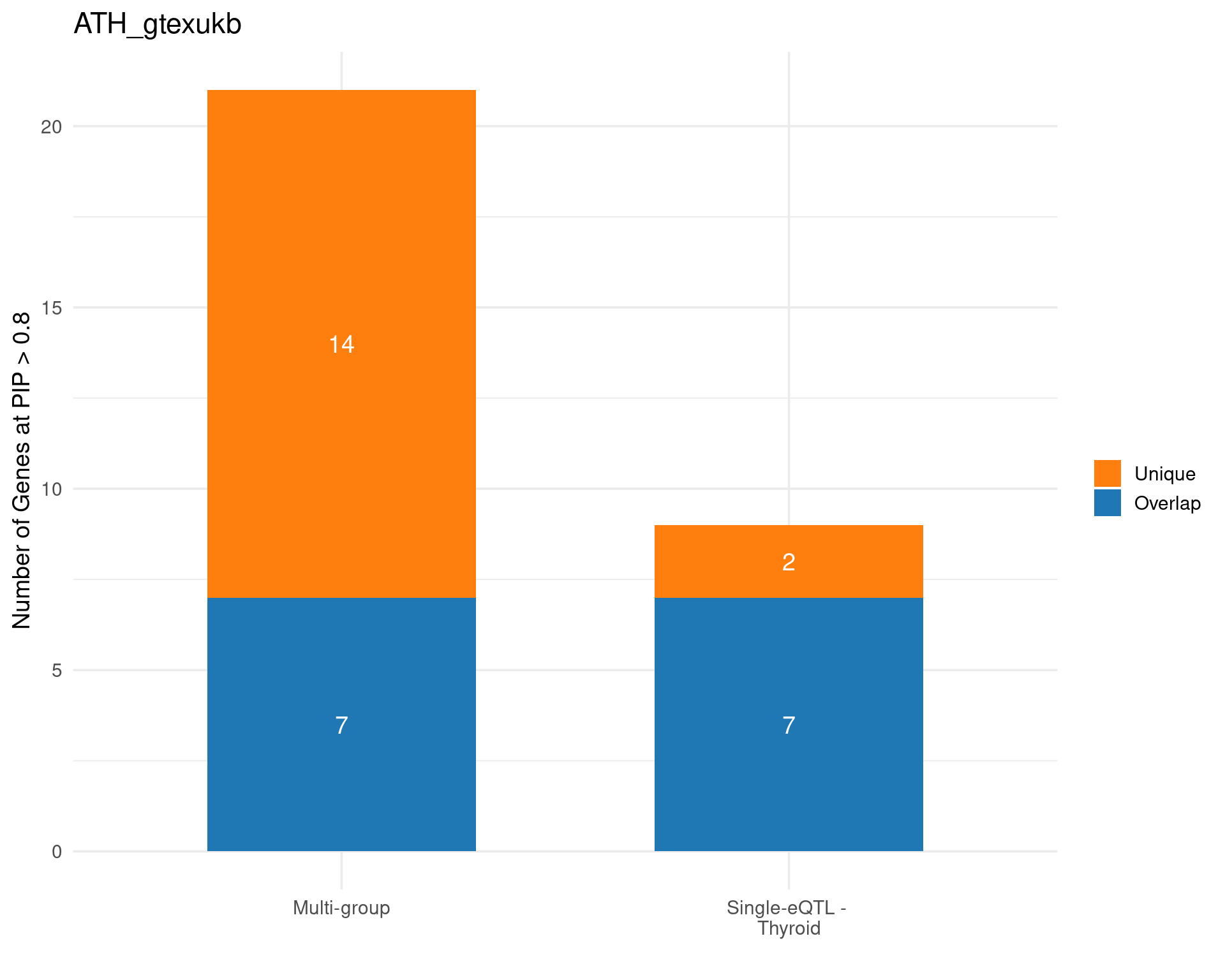
$single_genes_unique
[1] "ZDHHC24" "CEP95" 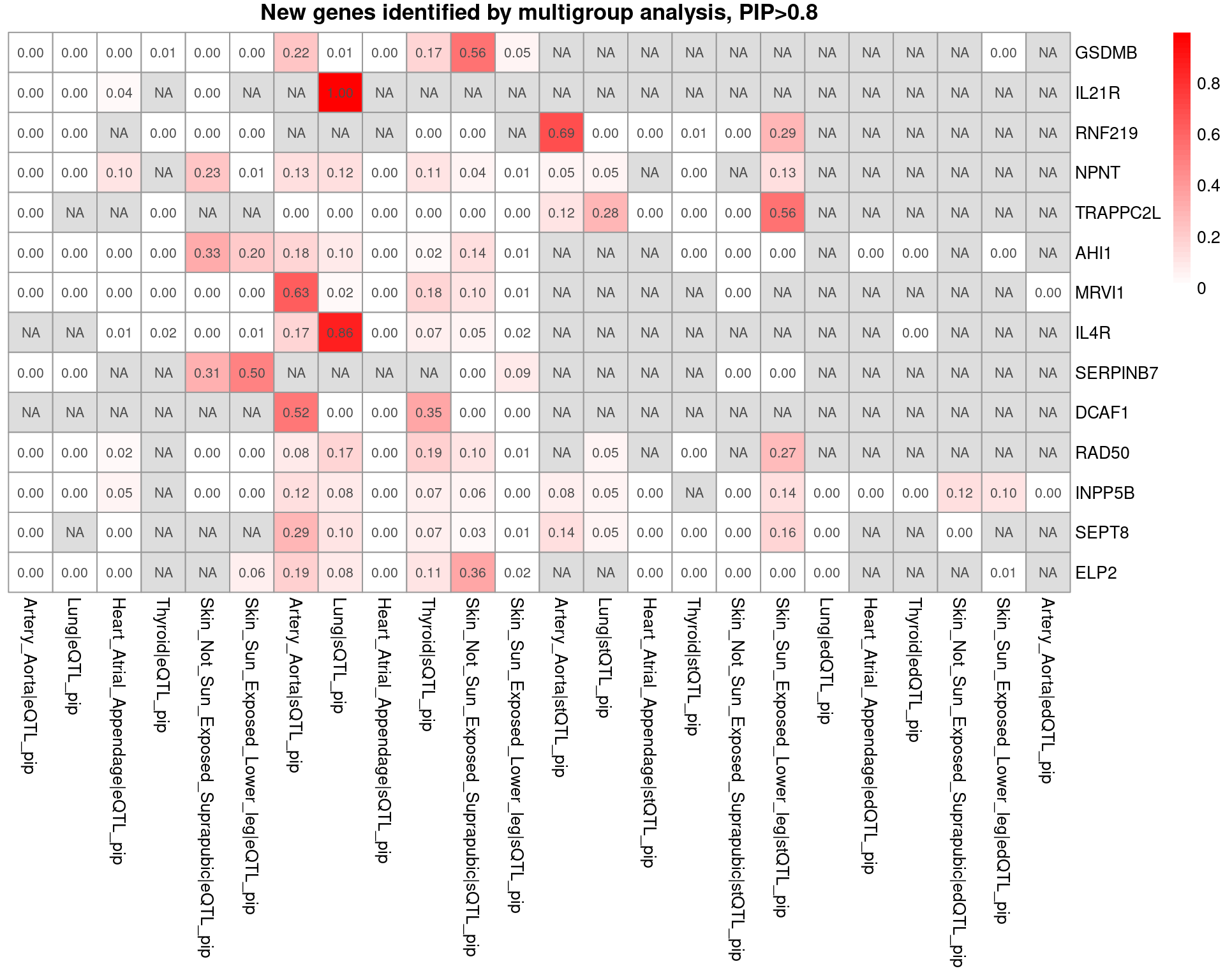
[1] "Unique genes from multigroup: GSDMB, IL21R, RNF219, NPNT, TRAPPC2L, AHI1, MRVI1, IL4R, SERPINB7, DCAF1, RAD50, INPP5B, SEPT8, ELP2"

BMI-panukb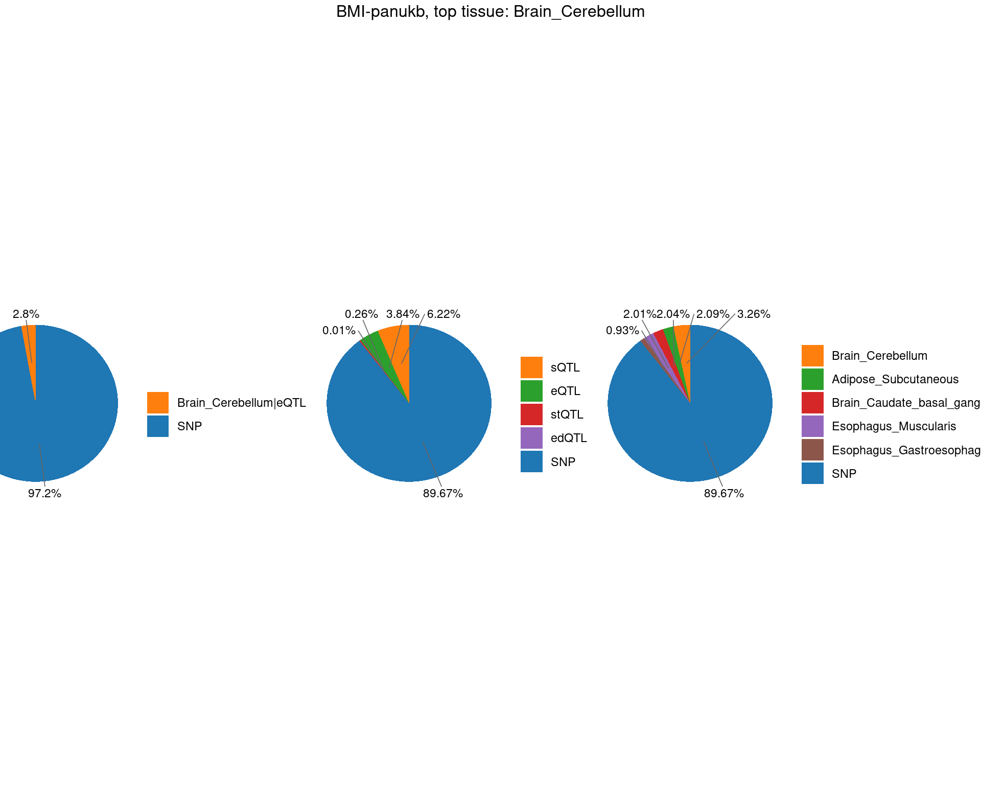
TableGrob (2 x 3) "arrange": 4 grobs
  z     cells    name                 grob
1 1 (2-2,1-1) arrange       gtable[layout]
2 2 (2-2,2-2) arrange       gtable[layout]
3 3 (2-2,3-3) arrange       gtable[layout]
4 4 (1-1,1-3) arrange text[GRID.text.1647]
$plot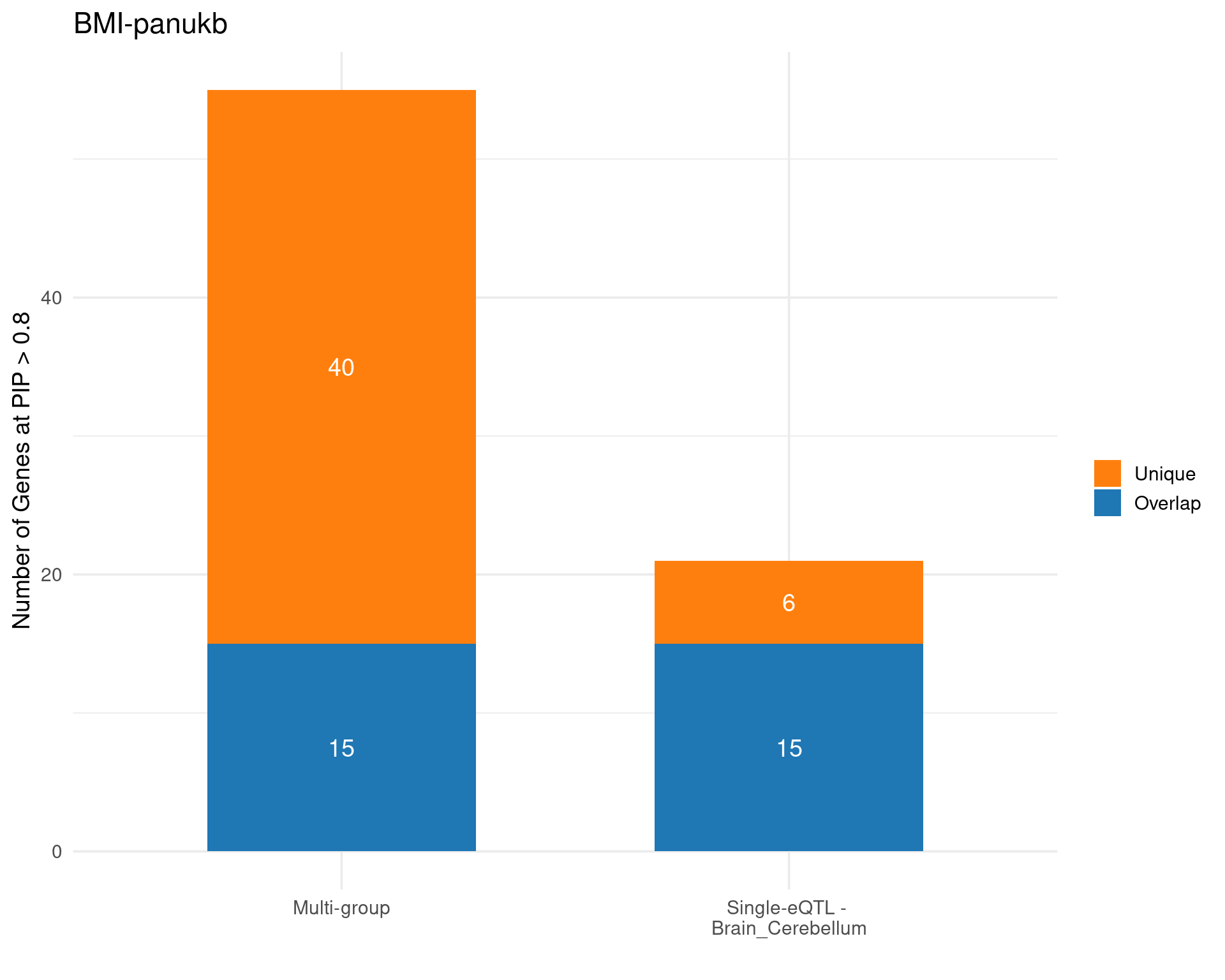
$single_genes_unique
[1] "PSORS1C1" "MAPK11" "ENHO" "C1QTNF4" "FAM231B" "DLG4" 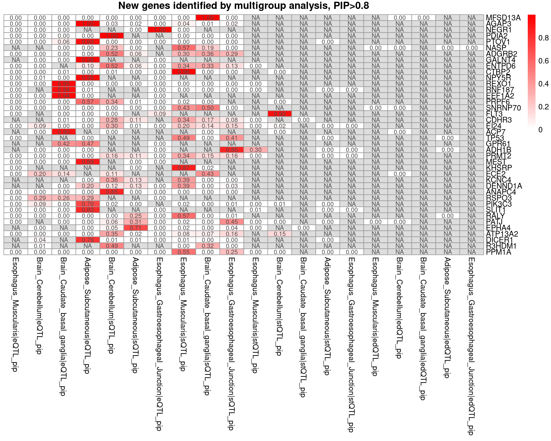
[1] "Unique genes from multigroup: MFSD13A, AGAP3, NEGR1, PDIA2, PTOV1, NASP, ADGRB2, GALNT4, ENTPD6, CTBP2, NPY5R, REXO1, RNF187, EEF1A2, PRPF6, SNRNP70, FLT3, CDHR3, EI24, ACP7, TP53, GPR61, ADH1B, PRMT2, MEST, KHSRP, ECE2, KCNC4, DENND1A, ANAPC4, RSPO3, PIK3C3, SLIT1, RALY, PATJ, EPHA4, ATP13A2, DICER1, R3HDM1, PPM1A"

HB-panukb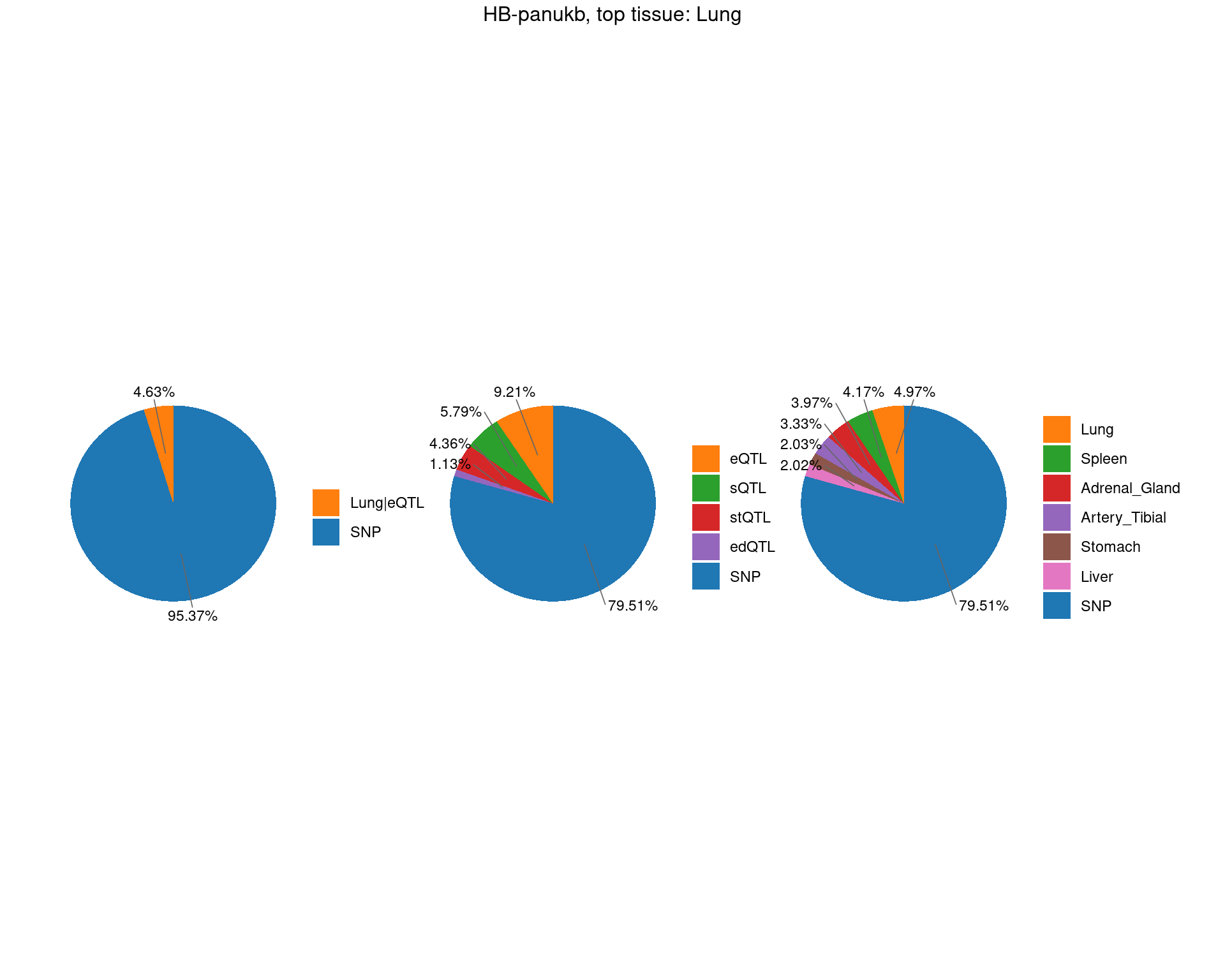
TableGrob (2 x 3) "arrange": 4 grobs
  z     cells    name                 grob
1 1 (2-2,1-1) arrange       gtable[layout]
2 2 (2-2,2-2) arrange       gtable[layout]
3 3 (2-2,3-3) arrange       gtable[layout]
4 4 (1-1,1-3) arrange text[GRID.text.1861]
$plot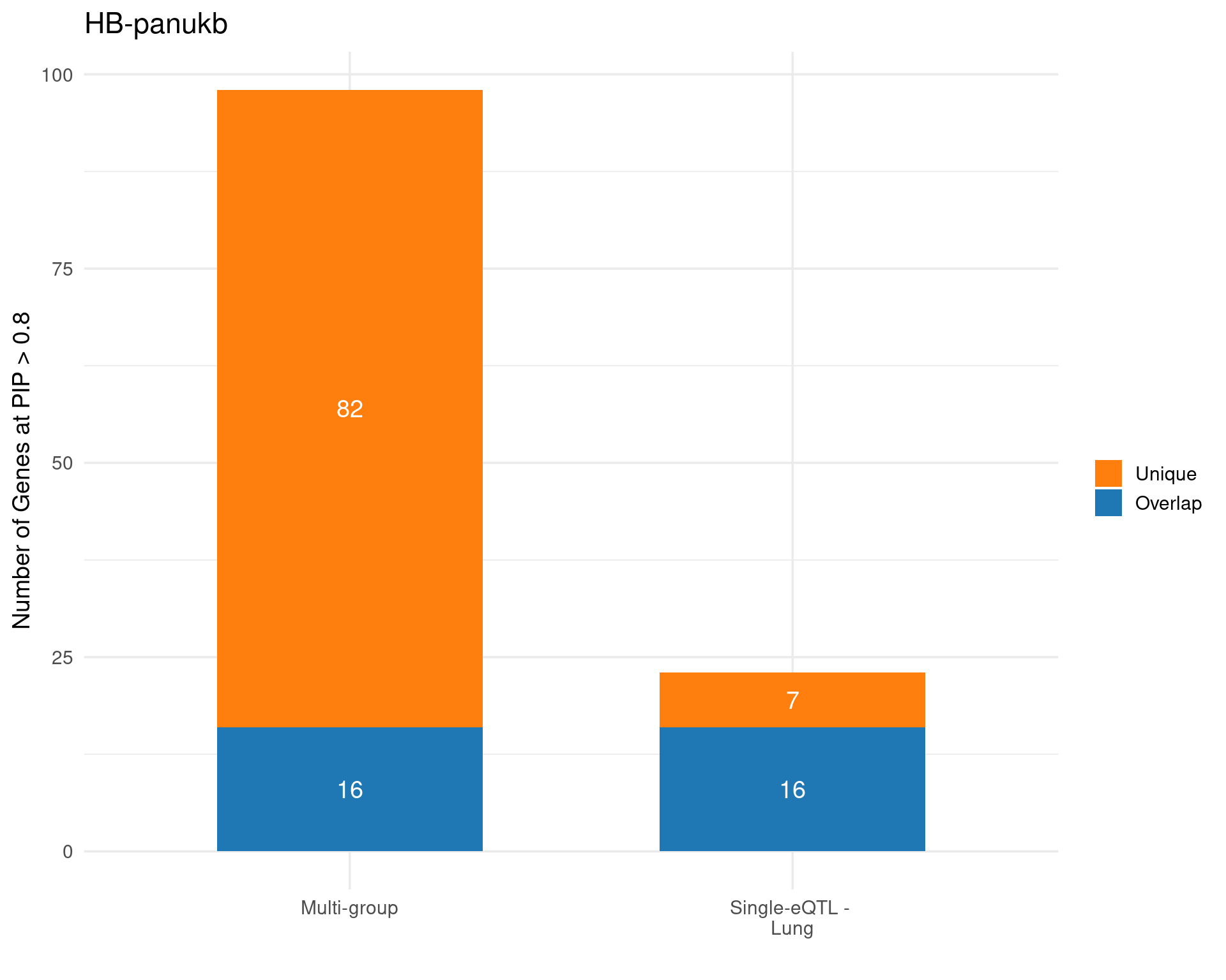
$single_genes_unique
[1] "MKRN2OS" "ENTPD6" "KIFC2" "PPP5C" "CCND2" "SH3GL1" "PLA2G6" 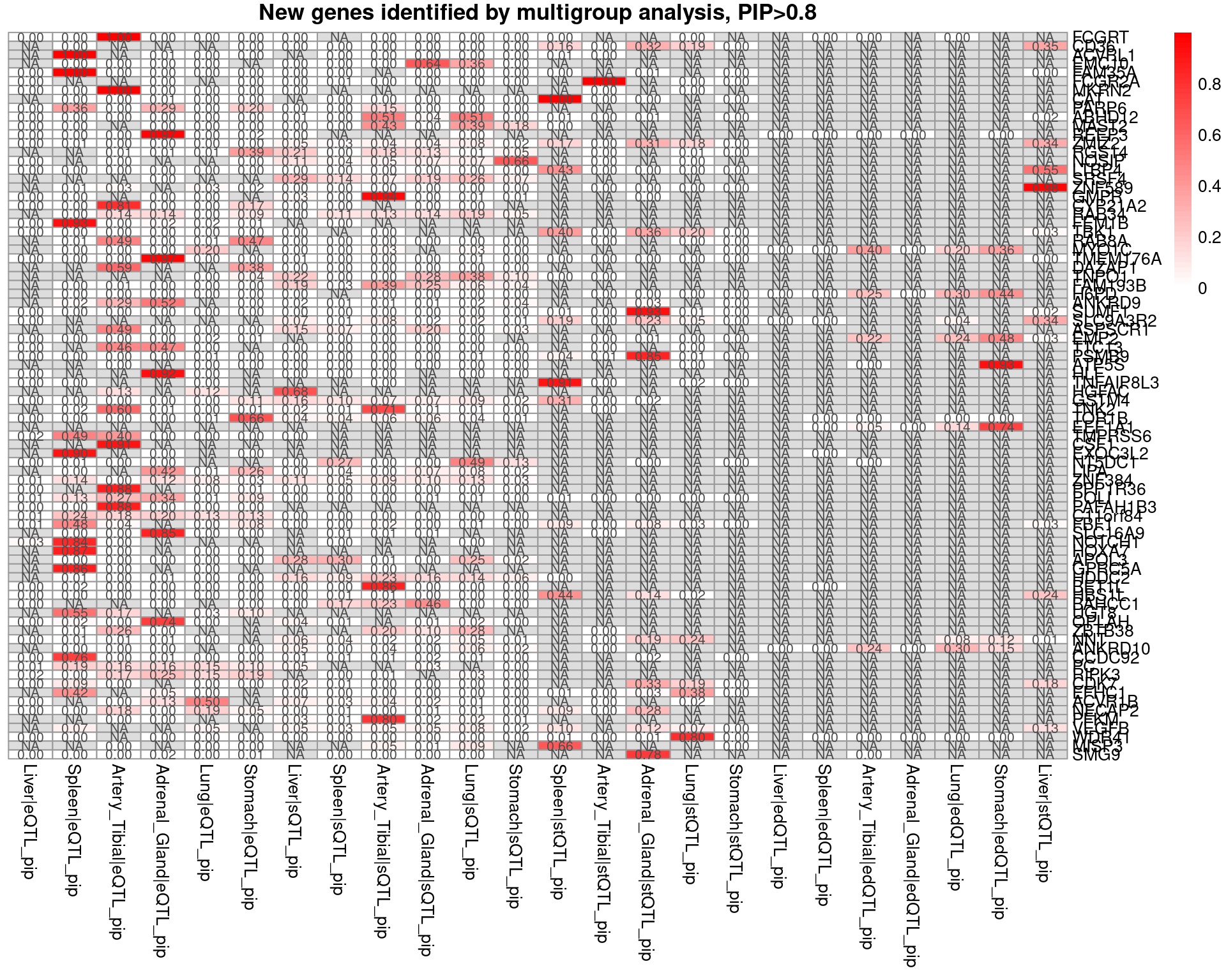
[1] "Unique genes from multigroup: FCGRT, CD36, ACVRL1, EMC10, FAM35A, FCGR2A, MKRN2, CAT, PARP6, ABHD12, MAST2, REEP3, ZMIZ2, RGS14, NOSIP, LTBP4, SRSF4, ZNF589, GMPR, CYP21A2, RAB34, FEM1B, TBK1, RAB8A, MYO1C, TMEM176A, DAZAP1, TNPO1, FAM193B, H6PD, ANKRD9, SUMF1, SLC9A3R2, ASPSCR1, EMP2, TTC13, PSMB9, ATP5S, HLF, TNFAIP8L3, HGFAC, GSTM4, TNK2, TOR1B, EEF1A1, TMPRSS6, CSF1, EXOC3L2, NT5DC1, LIPA, ZNF384, PPP1R36, POLI, PAFAH1B3, C11orf84, FBF1, SLC16A9, NOTCH1, HOXA7, APOL3, GPRC5A, HDDC2, BET1L, HBS1L, BAHCC1, UGT8, OPLAH, ZBTB38, NNT, ANKRD10, CCDC92, PC, RIPK3, CDK7, EFHC1, ACVR1B, NECAP2, PFKM, VEGFB, WDR41, MISP3, SMG9"

Height-panukb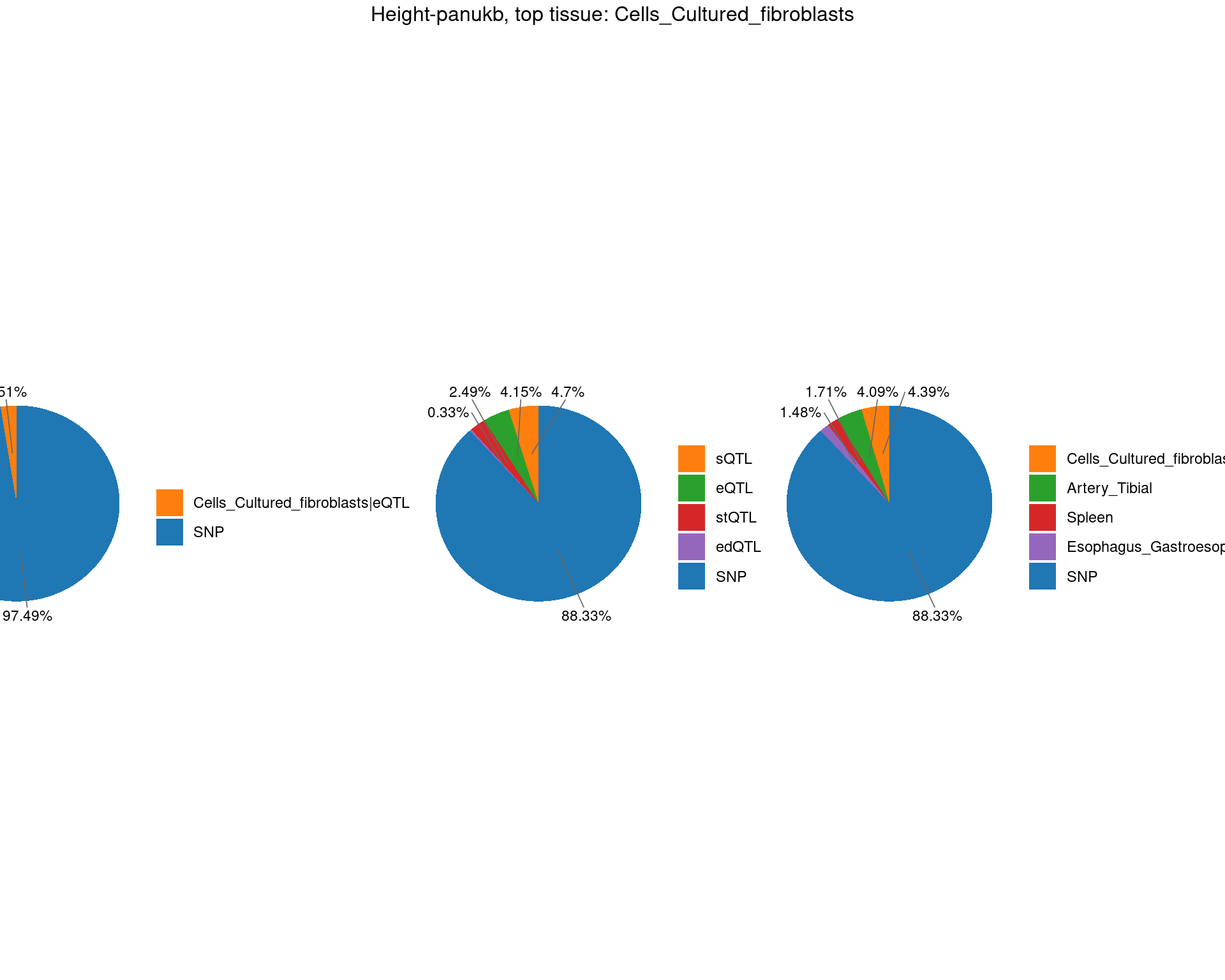
TableGrob (2 x 3) "arrange": 4 grobs
  z     cells    name                 grob
1 1 (2-2,1-1) arrange       gtable[layout]
2 2 (2-2,2-2) arrange       gtable[layout]
3 3 (2-2,3-3) arrange       gtable[layout]
4 4 (1-1,1-3) arrange text[GRID.text.2068]
$plot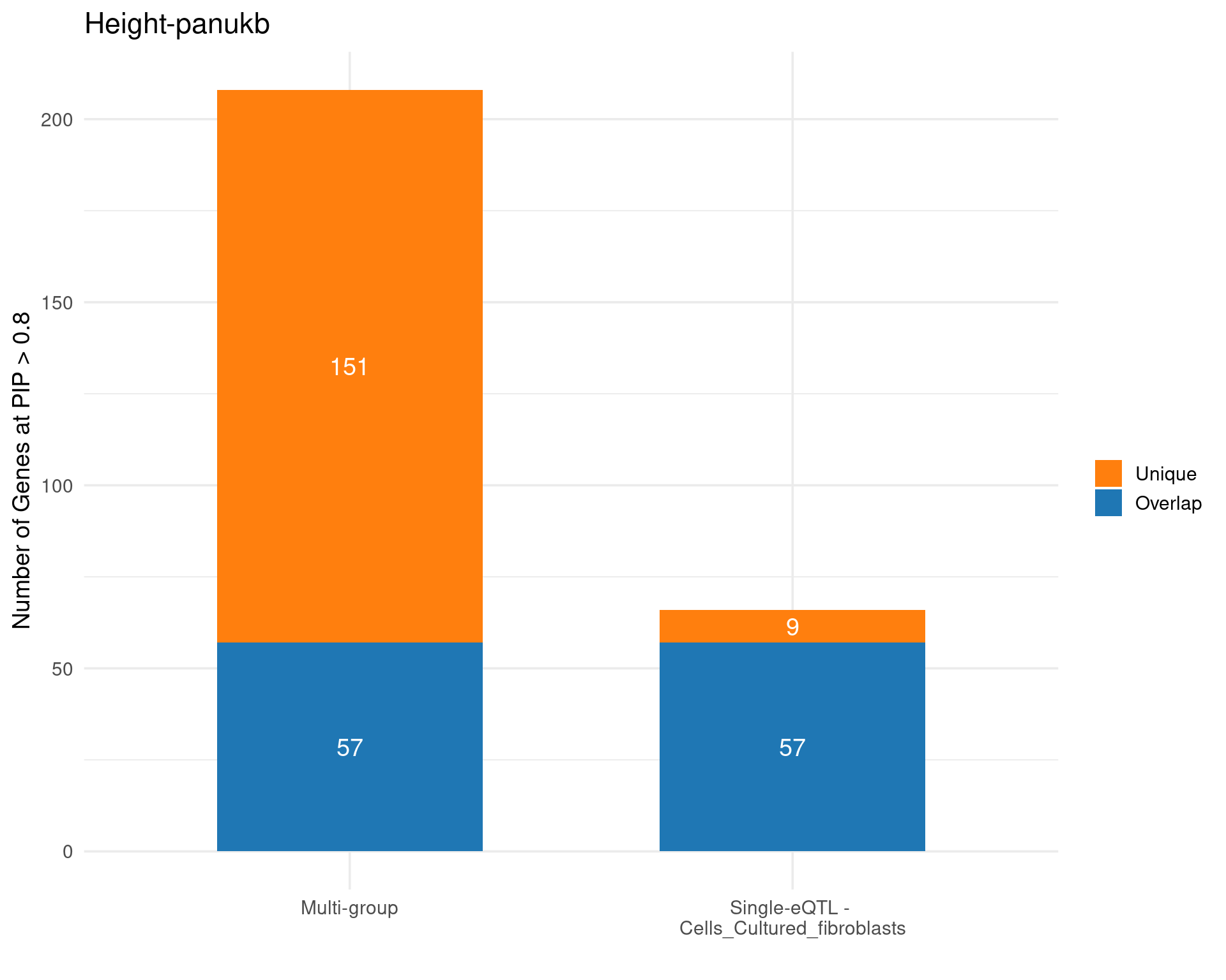
$single_genes_unique
[1] "RGP1"       "ACHE"       "SRSF12"     "DVL3"       "SPHK2"
[6] "PSMB9" "TOPORS-AS1" "UTP11" "MYLK4" 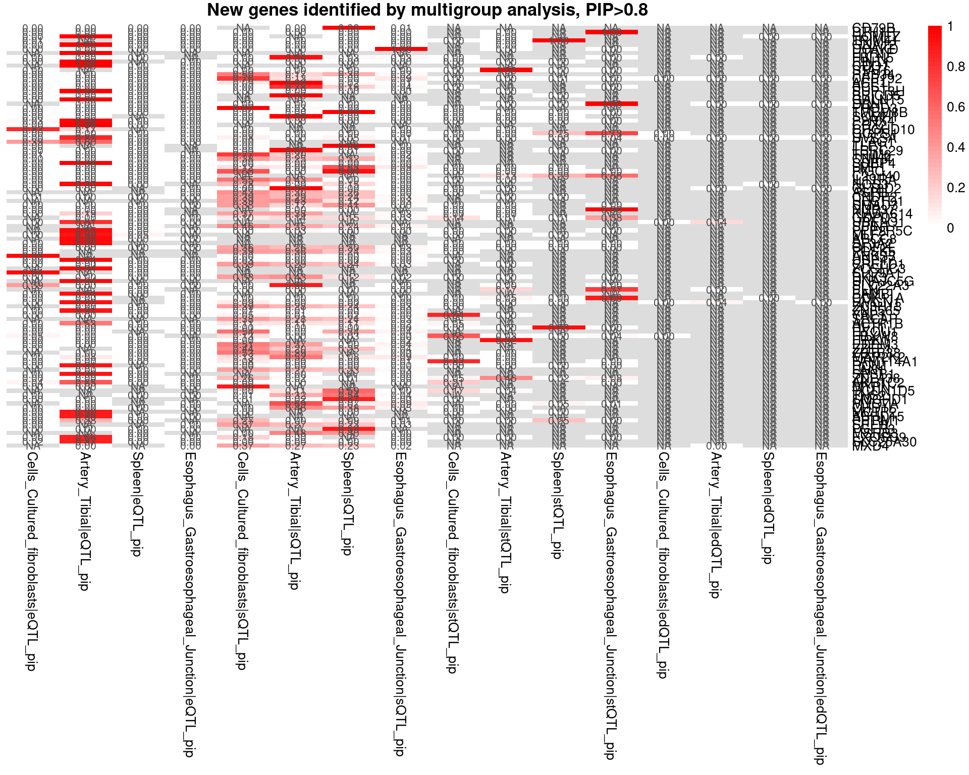
[1] "Unique genes from multigroup: CD79B, PTH1R, HOMEZ, TRIM41, GNA12, DCAKD, HTR1F, FBLN5, RINT1, CDO1, STAT6, RAB34, CEP192, ACP1, BCS1L, SUPT3H, BRICD5, GALNT5, DBNL, FHOD3, TMEM8B, SCMH1, P2RX4, CBX2, CHCHD10, GGPS1, UVSSA, PLAG1, TLE1, LRRC29, TRIM6, CNIH4, SSBP4, LMF1, PIGC, C2orf40, IL11RA, NOS3, GLT8D2, ASPH, CNDP2, HECTD1, SMAD3, NUP37, KIAA1614, GDPD3, UBE2Q1, SPIN1, PPP2R5C, MLF2, ABCC8, SF3A2, ODF2L, PCSK5, ANKS3, USP47, CRELD1, ZCCHC3, SLC9A1, DKK3, DNAJC5G, SLC22A3, ELN, BAMBI, CDK11A, HMGN1, ZC3H13, ZNF565, YAP1, SRCAP, ACTR1B, RFT1, HYOU1, FBXW8, ITPK1, EDEM3, ZZEF1, ZBTB38, MAP2K2, FAM114A1, RCN1, FAN1, SPSB1, ZNF438, AKR1C2, MYPN, DCUN1D5, TNS2, SMCHD1, MYO7A, CHD1L, MCTP2, ABHD15, PITRM1, SEL1L, FGFR3, MSRB3, EXOSC9, SLC25A30, MXD4, TTLL6, RALGAPA2, PARP12, TPRG1L, FAM134B, DAAM2, CCND3, ZNF484, SZT2, CKB, RBCK1, EIF3C, TRPS1, ARSJ, ARL15, GSDMC, ARHGAP24, ZMIZ2, SLC25A32, NCR3LG1, SEC23IP, ZBP1, VAMP5, FUBP3, RDH10, RPS6KA4, LUC7L2, ATP10D, PAPD4, SLC48A1, KCNJ12, RREB1, SAMD4A, CTU2, CCDC57, RPS9, SOCS1, UST, SSR3, FN3KRP, MMAB, VMAC, PSMF1, HNRNPC, MORC3, MPHOSPH6, SERPINH1, ATP1B3, GATAD2A, ASPSCR1, CREB3L2"

HTN-panukb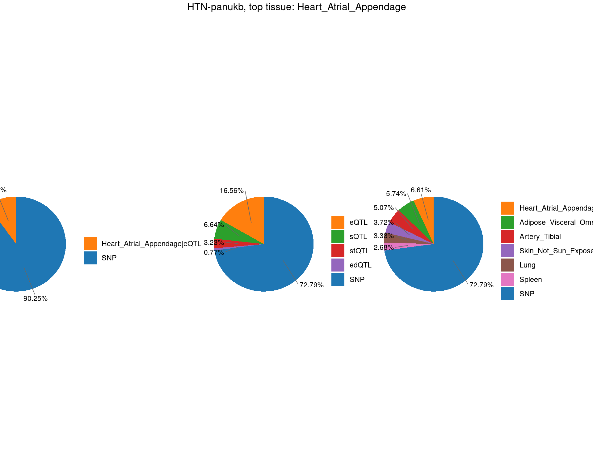
TableGrob (2 x 3) "arrange": 4 grobs
  z     cells    name                 grob
1 1 (2-2,1-1) arrange       gtable[layout]
2 2 (2-2,2-2) arrange       gtable[layout]
3 3 (2-2,3-3) arrange       gtable[layout]
4 4 (1-1,1-3) arrange text[GRID.text.2281]
$plot
$single_genes_unique
[1] "TAPBP"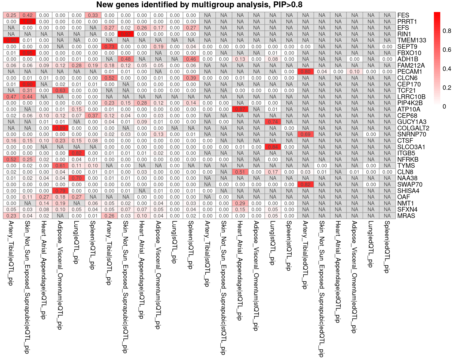
[1] "Unique genes from multigroup: FES, PRRT1, EFS, RIN1, TMEM133, SEPT9, FBXO10, ADH1B, FAM212A, PECAM1, CLCN6, CEP170, TCF21, LRRC10B, PIP4K2B, ATP10A, CEP68, GUCY1A3, COLGALT2, SNRNP70, CTSF, SLCO3A1, ITGB5, NFRKB, TYMS, CLN8, NAA38, SWAP70, SHISA4, OAF, NMT1, SFXN4, MRAS"

PLT-panukb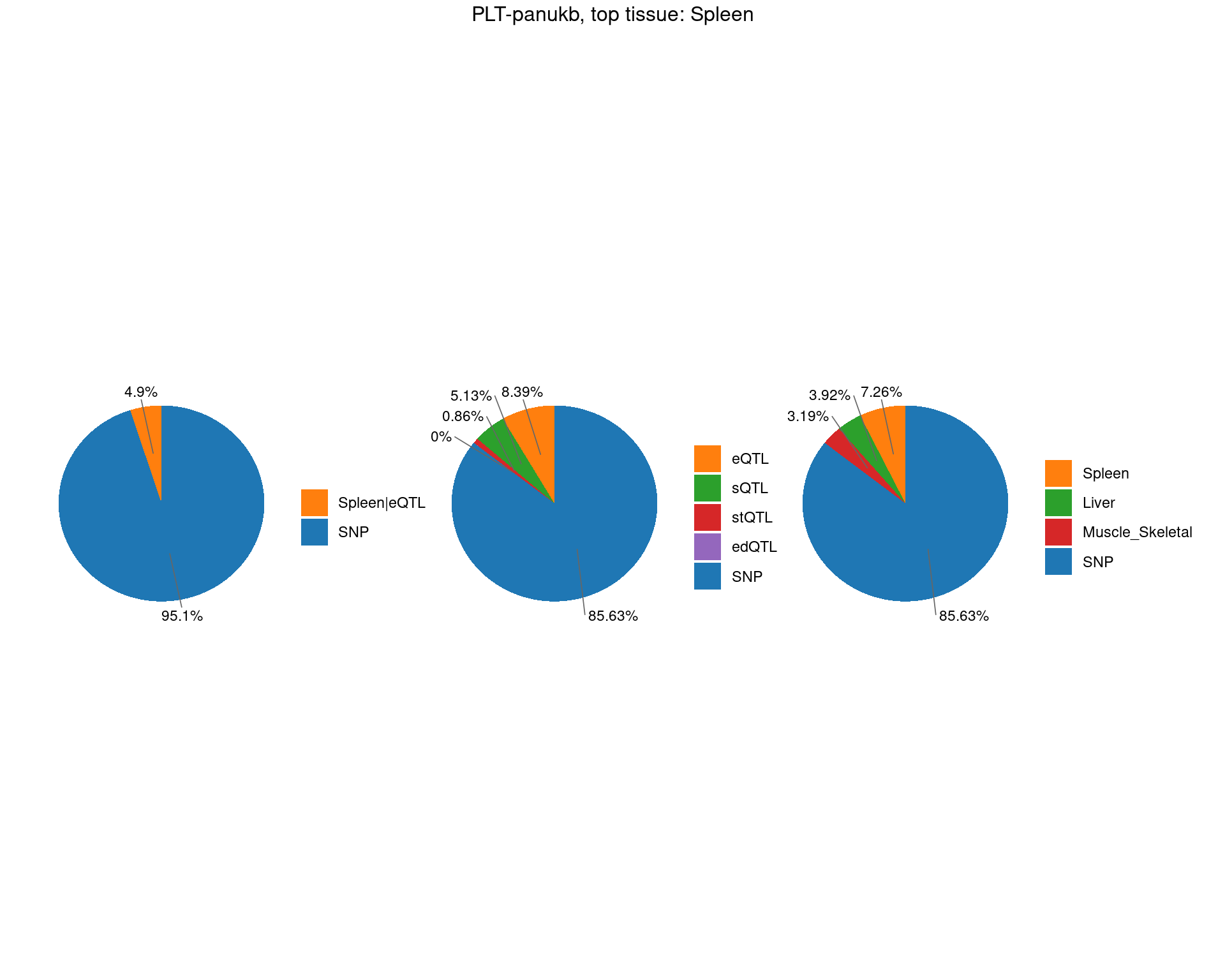
TableGrob (2 x 3) "arrange": 4 grobs
  z     cells    name                 grob
1 1 (2-2,1-1) arrange       gtable[layout]
2 2 (2-2,2-2) arrange       gtable[layout]
3 3 (2-2,3-3) arrange       gtable[layout]
4 4 (1-1,1-3) arrange text[GRID.text.2484]
$plot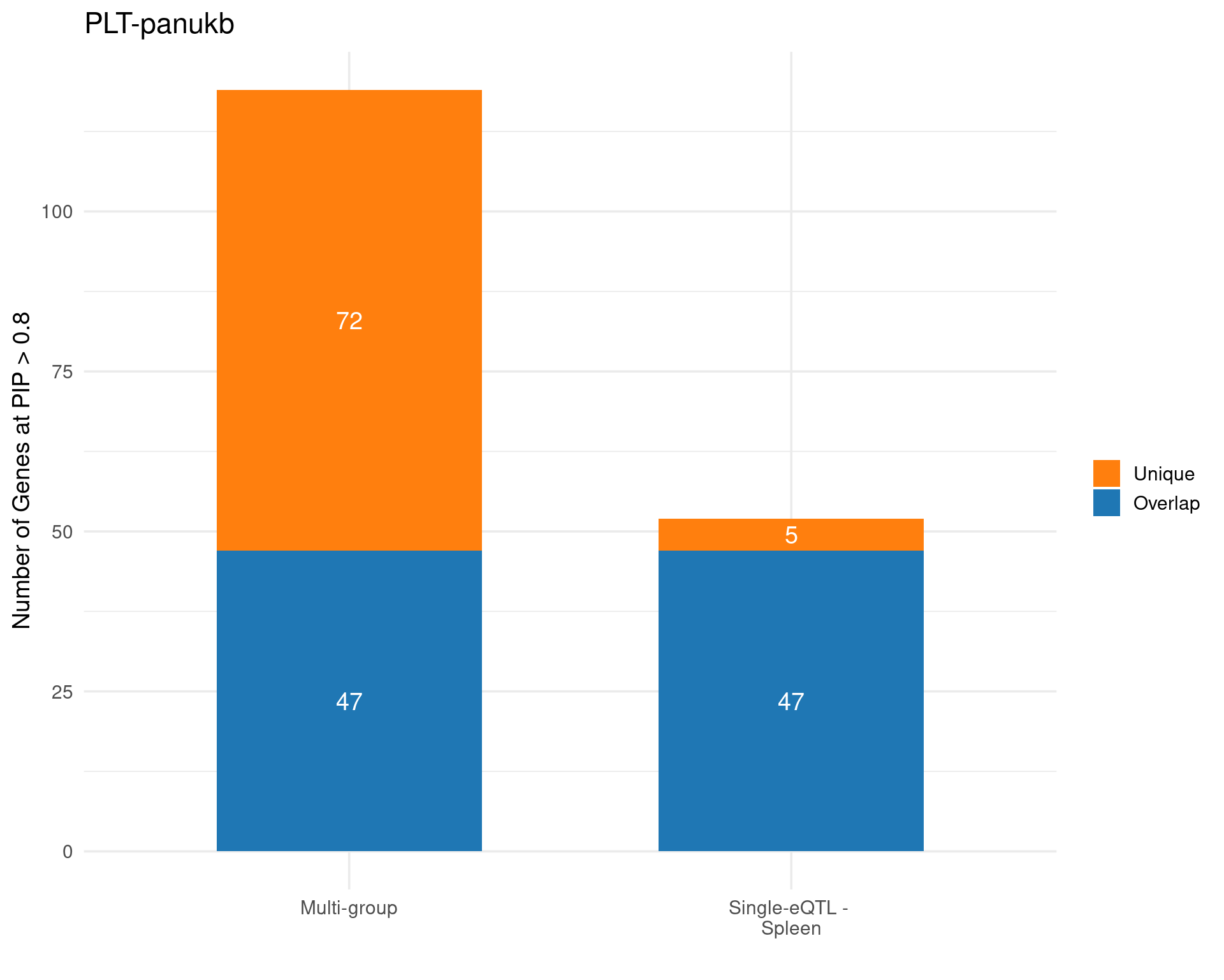
$single_genes_unique
[1] "WBP2" "TRABD" "HPR" "HNRNPUL1" "JADE2" 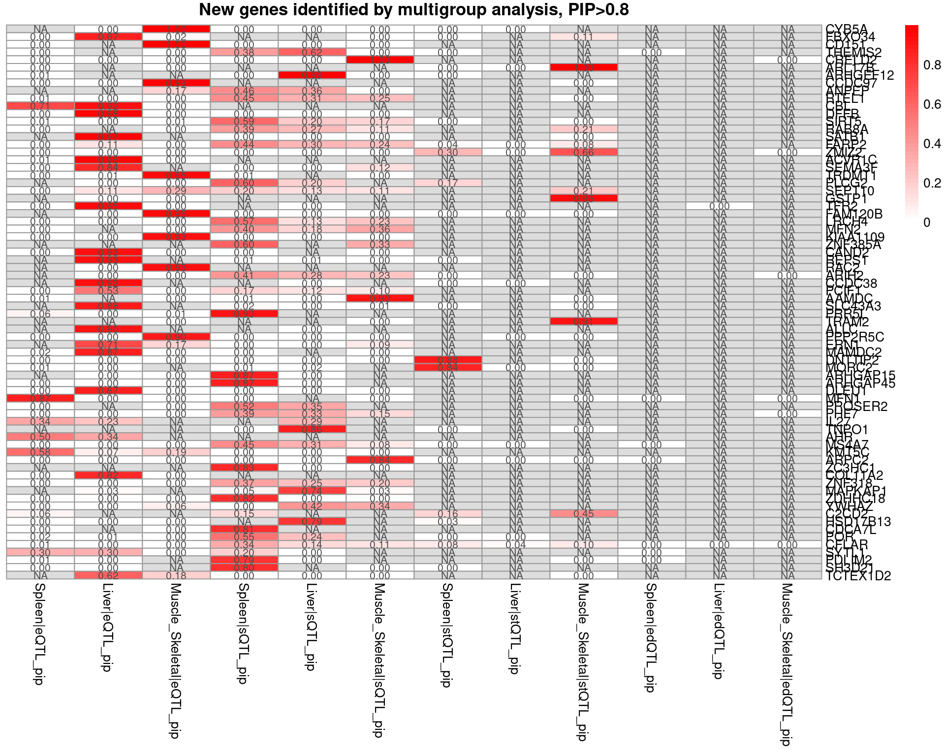
[1] "Unique genes from multigroup: CYB5A, FBXO34, CD151, THEMIS2, CRELD2, ARL17B, ARHGEF12, CCDC97, ANPEP, RTEL1, CBL, DFFB, SIRT5, RAB8A, SATB1, FARP2, ZMIZ2, ACVR1C, SEMA3F, TRDMT1, PLCG2, SEPT10, GSTP1, TFR2, FAM120B, LRCH4, MFN2, KIAA1109, ZNF385A, CAND2, REPS1, RAC2, ARIH2, CCDC38, PCIF1, AAMDC, SLC43A3, PRR5L, TRAM2, ALLC, PPP2R5C, ERN1, MAMDC2, DNTTIP2, MORC2, ARHGAP15, ARHGAP45, DLEU1, MFN1, PROSER2, PHF7, IL27, TNPO1, AHR, MS4A7, KMT5C, ARPC2, ZC3HC1, COL11A2, ZNF318, MAPKAP1, ZDHHC18, YWHAZ, C2CD2, HSD17B13, CDCA7L, POR, CFLAR, SYTL1, PDLIM2, SH3D21, TCTEX1D2"

RA-panukb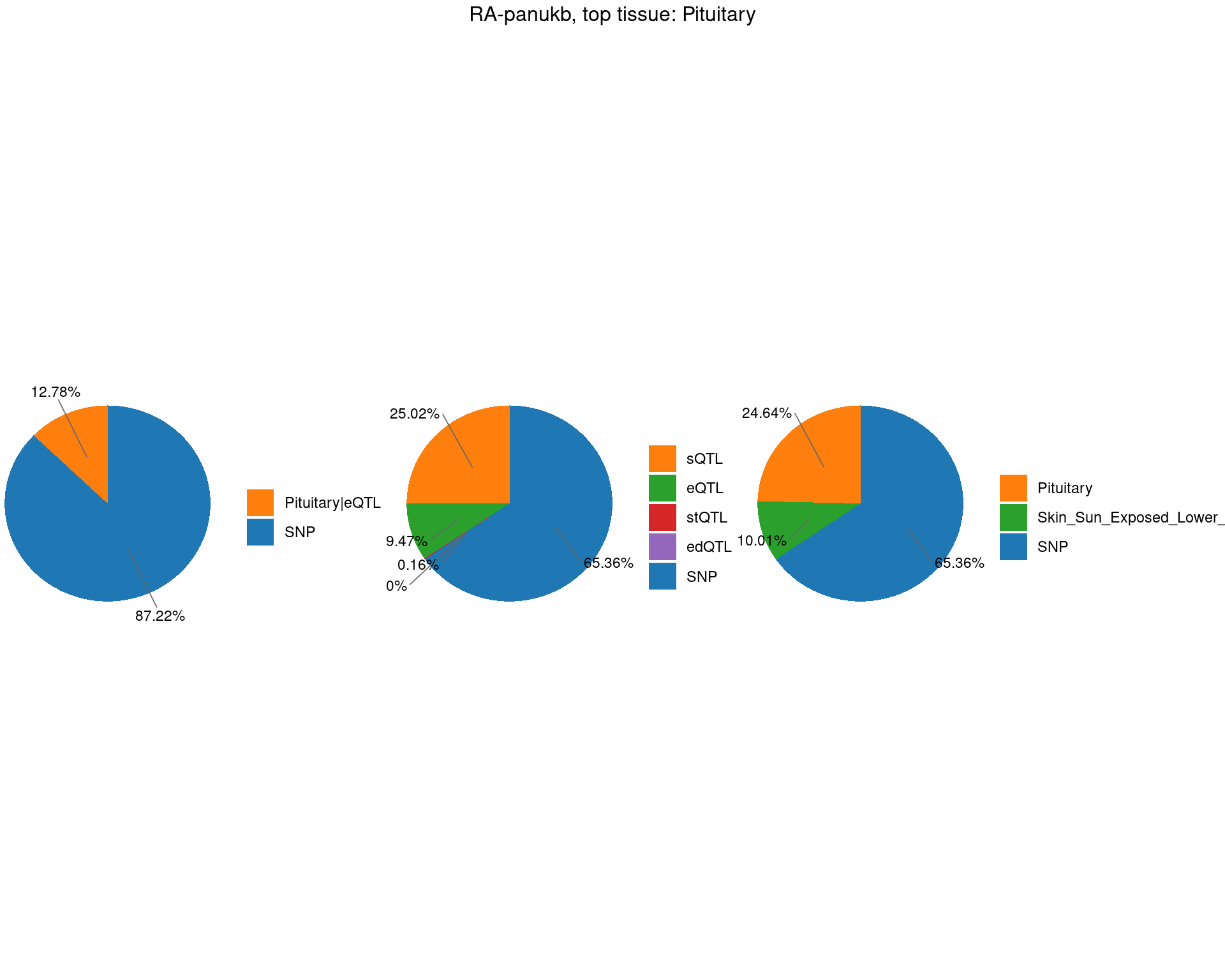
TableGrob (2 x 3) "arrange": 4 grobs
  z     cells    name                 grob
1 1 (2-2,1-1) arrange       gtable[layout]
2 2 (2-2,2-2) arrange       gtable[layout]
3 3 (2-2,3-3) arrange       gtable[layout]
4 4 (1-1,1-3) arrange text[GRID.text.2680]
$plot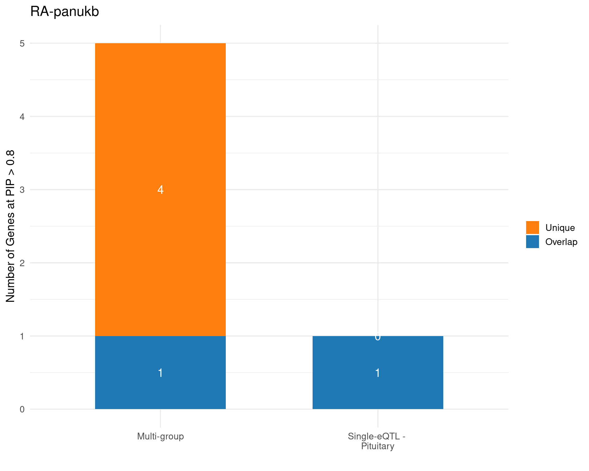
$single_genes_unique
character(0)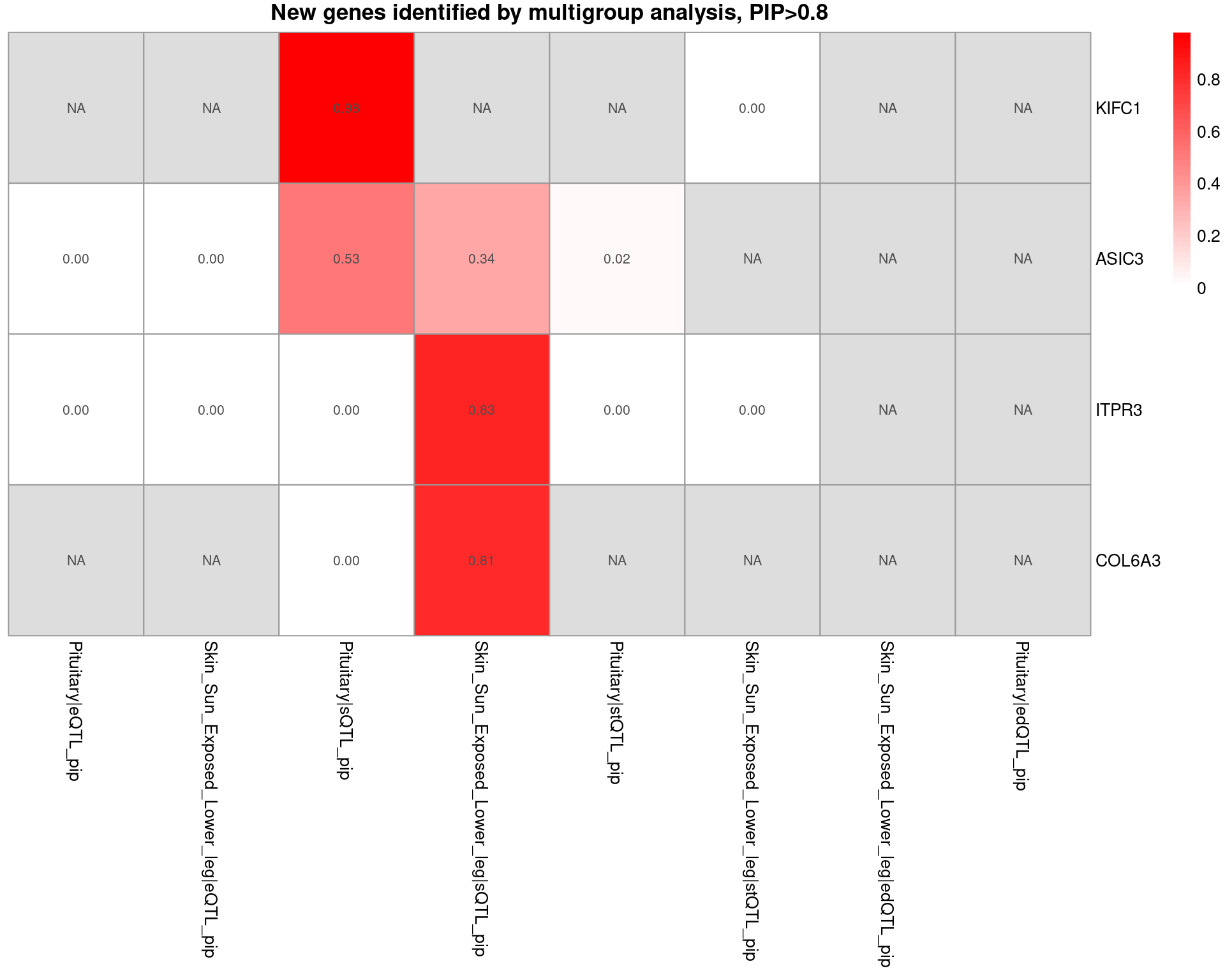
[1] "Unique genes from multigroup: KIFC1, ASIC3, ITPR3, COL6A3"

RBC-panukb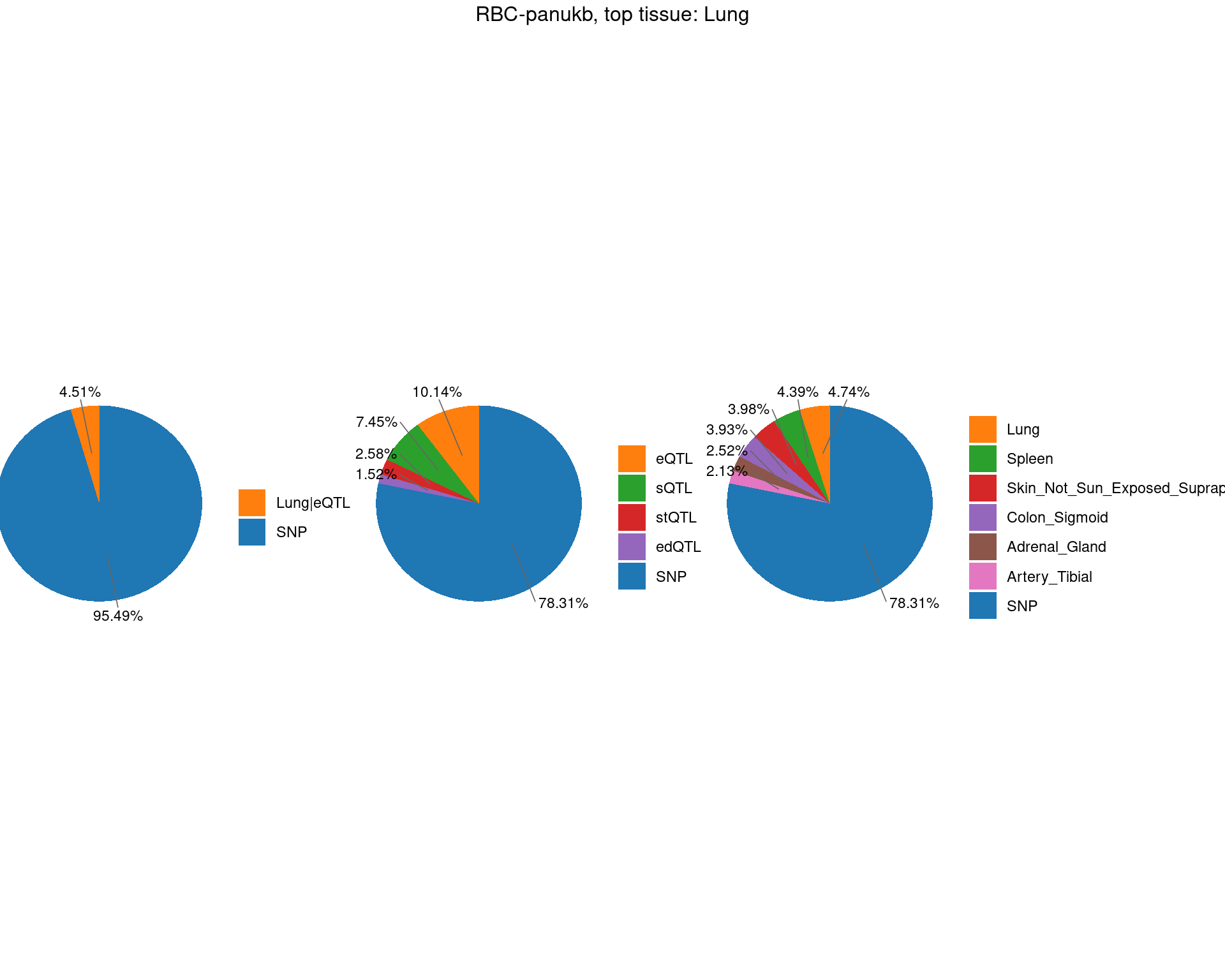
TableGrob (2 x 3) "arrange": 4 grobs
  z     cells    name                 grob
1 1 (2-2,1-1) arrange       gtable[layout]
2 2 (2-2,2-2) arrange       gtable[layout]
3 3 (2-2,3-3) arrange       gtable[layout]
4 4 (1-1,1-3) arrange text[GRID.text.2891]
$plot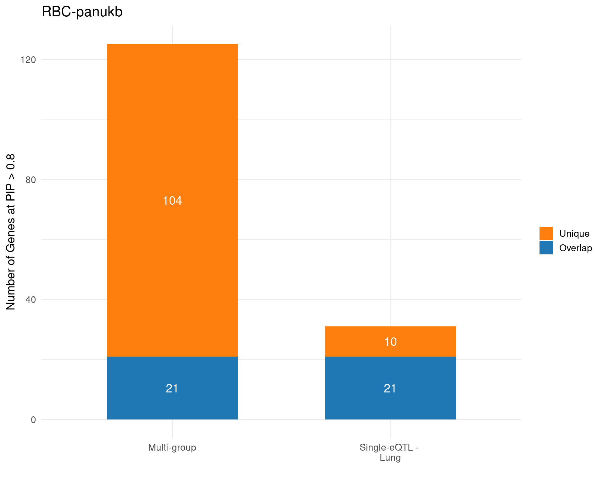
$single_genes_unique
 [1] "HLA-E"   "LRRC37A" "BST1"    "ESRRB"   "JMJD1C"  "PPP1R26" "H1F0"
[8] "PTPA" "MAPK3" "ZNF629" 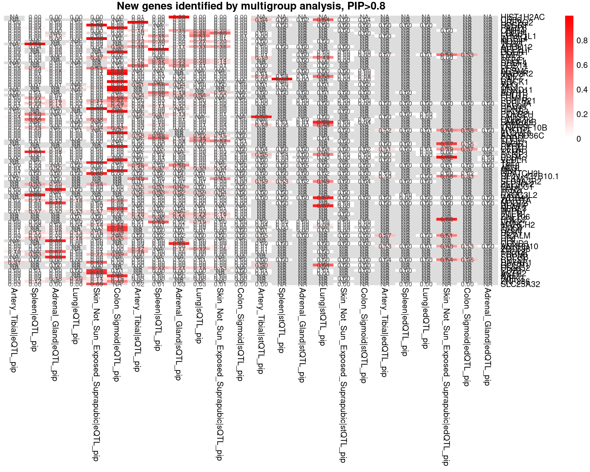
[1] "Unique genes from multigroup: HIST1H2AC, CD36, UBE2Q2, FCGRT, PARP6, CNIH4, LRCH4, EHBP1L1, INTS14, NOSIP, TFRC, ABHD12, NFE2L1, OSER1, EMP2, TP53, RTEL1, SRSF4, RGS14, FES, ACSM5, MAP2K2, ZMIZ2, CAT, ROCK1, XPC, TAL1, HOXD11, ADH1B, FHL3, FEM1B, PPP1R21, SPPL2A, RAB34, EDN1, PIK3R3, POLR2H, FADS1, CCDC92, FAM200B, PSMB5, TNFRSF10B, MYO1C, ELOVL3, ANKRD36C, PRR5L, TLE3, PIK3R1, RYBP, CFLAR, TYMS, PCGF3, PSD4, VLDLR, TST, TAF8, ADSL, MN1, GPATCH2L, RP11-437B10.1, PFKM, SLC9A3R2, ZFP36L2, BAHCC1, TFR2, ITSN1, EXOC3L2, WDR41, ZBTB7A, NUDT2, SLX4IP, NPRL3, TRPS1, PTEN, ZNF106, PQLC2, VRK2, MARCH2, TMC4, GLCE, DOK1, PICALM, RB1, HLF, CCND3, ANKRD10, ZBTB38, TTC13, PBRM1, SRPRB, CRLS1, DAZAP1, GOSR1, C6orf52, CD22, ACTR2, XAF1, RIPK3, ZNF236, SLC25A32, CRNN, DUS3L, UGT8, KANSL1"

WBC-ieu-b-30
TableGrob (2 x 3) "arrange": 4 grobs
  z     cells    name                 grob
1 1 (2-2,1-1) arrange       gtable[layout]
2 2 (2-2,2-2) arrange       gtable[layout]
3 3 (2-2,3-3) arrange       gtable[layout]
4 4 (1-1,1-3) arrange text[GRID.text.3114]
$plot
$single_genes_unique
 [1] "FCER1G" "ACAP1"  "APOBR"  "HPN"    "RNF181" "FOXJ2"  "GPN2"   "TIMM50"
[9] "TPST1" "JMJD6" "ABI3" "MARK2" "PSMD2" 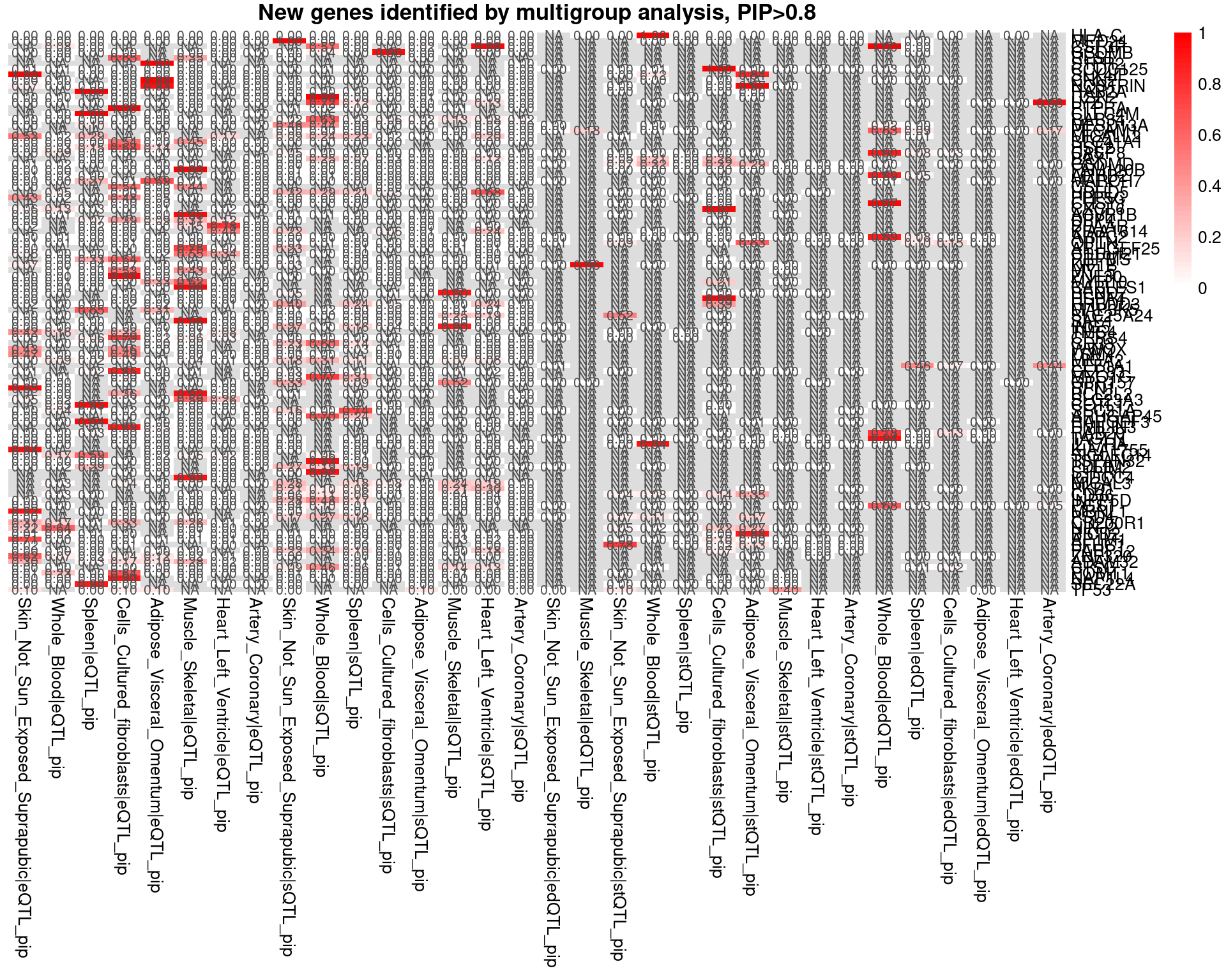
[1] "Unique genes from multigroup: HLA-C, MED24, CSF3R, GSDMB, REST, S1PR2, CCDC125, SLX4IP, CNN2, NOSTRIN, RAB2A, ITSN2, LYZ, PTPRA, CLEC4M, RAB34, MFSD13A, PECAM1, MICALL2, SLC41A1, HSF2, CASP8, BAX, GSDMD, FAM120B, ARRB2, MARCH7, CSF1, HDHD5, PPP5C, CHSY1, CXCL6, ACVR1B, DPP4, SPAAR, KIAA1614, ARPC2, OPTN, ARHGEF25, C11orf21, RBPMS, KIF1B, MYL5, ZNF30, MYH10, CABLES1, BEND7, HSPA4, RHBDD3, MAP3K5, SLC25A24, SAE1, ING5, TMC4, CERS4, CD33, WWOX, LSM4, MIGA2, EEF1A1, CEP83, MYO1G, GPR157, RPN1, BCL2L2, SLC23A3, COTL1, SEC31A, ARHGAP45, RAPGEF3, EMILIN3, RAB29, TAGLN, IL17RA, KIAA1755, SIGLEC14, TSPAN32, PDLIM2, S1PR1, IGDCC4, MICAL3, PKD1, CD36, INPP5D, PGS1, MBNL1, PSD4, CD200R1, NINJ2, BICD2, AP1M1, EFHC1, PARP12, ZNF320, ADAM32, CTSC, POMT1, NAP1L4, SEC22A, TP53, DSTN, FN1, MKRN2, ABCC5, RBM38, SCPEP1, ATL2, PLCG2, LIMS2, TSPAN14, ANKRD44, ATP11A, CARS2, PRR16, FLT3LG, IRF5, MAP3K10, CACNA1H, CTDSPL, UPP1, MAPK14, CD300A, CSGALNACT1, SCD, ZNF713, FYCO1, CAPZB, VSIR, ZC3H12D, WDR86, MYO1C, LRBA, CD226, ZFP1, CEPT1, EIF4E2, SUSD1, TET2, VPS16, AMZ1, RNF139, ITGB2, PAPSS1, IL16, AKAP11, B4GALT3, CREB3L3, AMPD1, TBC1D10C, CCDC82, HEATR3, DLG5, ARHGAP31, SBNO2, SNX32, GOLGA5, CD46, TRAP1, GADD45G, TBX2, IFNAR1, ACKR2, DTNB, ZNF461, DEFB1, HOXC6, NPAS2, NUDT14, ZC3HC1, SLC45A4, RAP1GAP2, FIGNL1, SLC39A9, FBXO38, TRAF3IP3, TM7SF3, NOC3L, TBL2, UGDH, MAP3K7CL, ELMO1"

SCZ-ieu-b-5102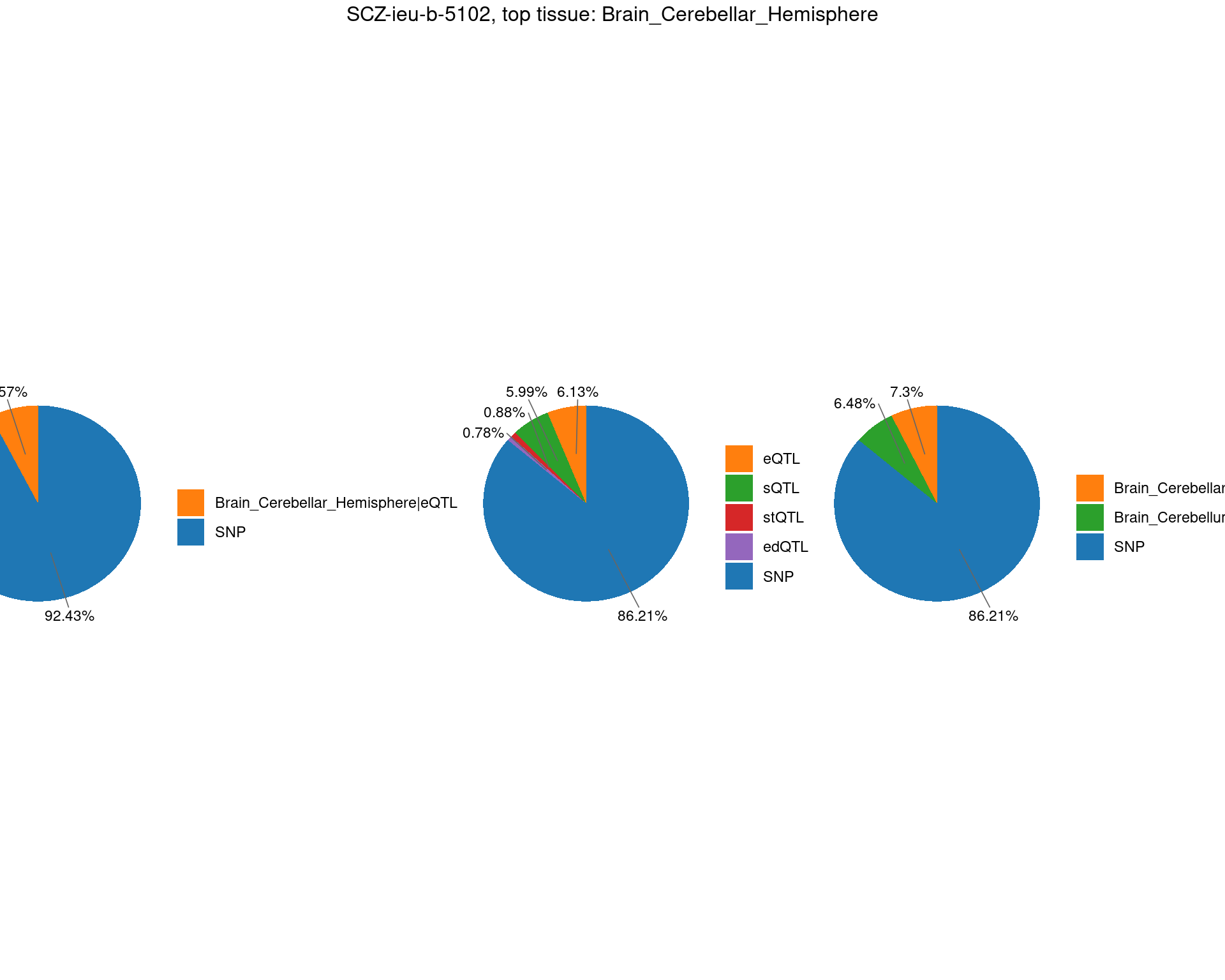
TableGrob (2 x 3) "arrange": 4 grobs
  z     cells    name                 grob
1 1 (2-2,1-1) arrange       gtable[layout]
2 2 (2-2,2-2) arrange       gtable[layout]
3 3 (2-2,3-3) arrange       gtable[layout]
4 4 (1-1,1-3) arrange text[GRID.text.3315]
$plot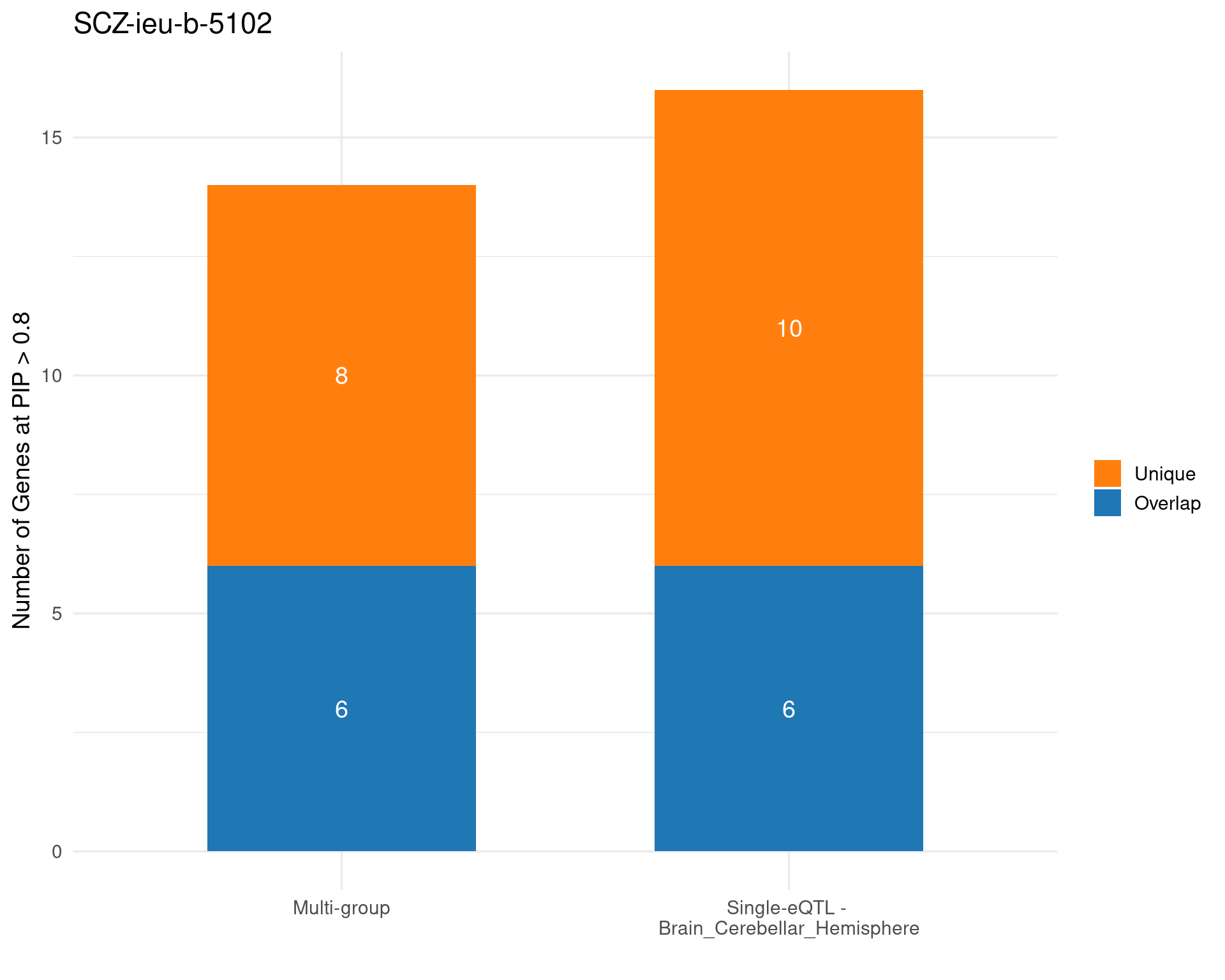
$single_genes_unique
 [1] "SLC38A3"  "HLA-DMB"  "TMEM222"  "KLHL20"   "DRD2"     "LY6H"
[7] "TRMT2A" "MLF2" "C11orf80" "PUF60" 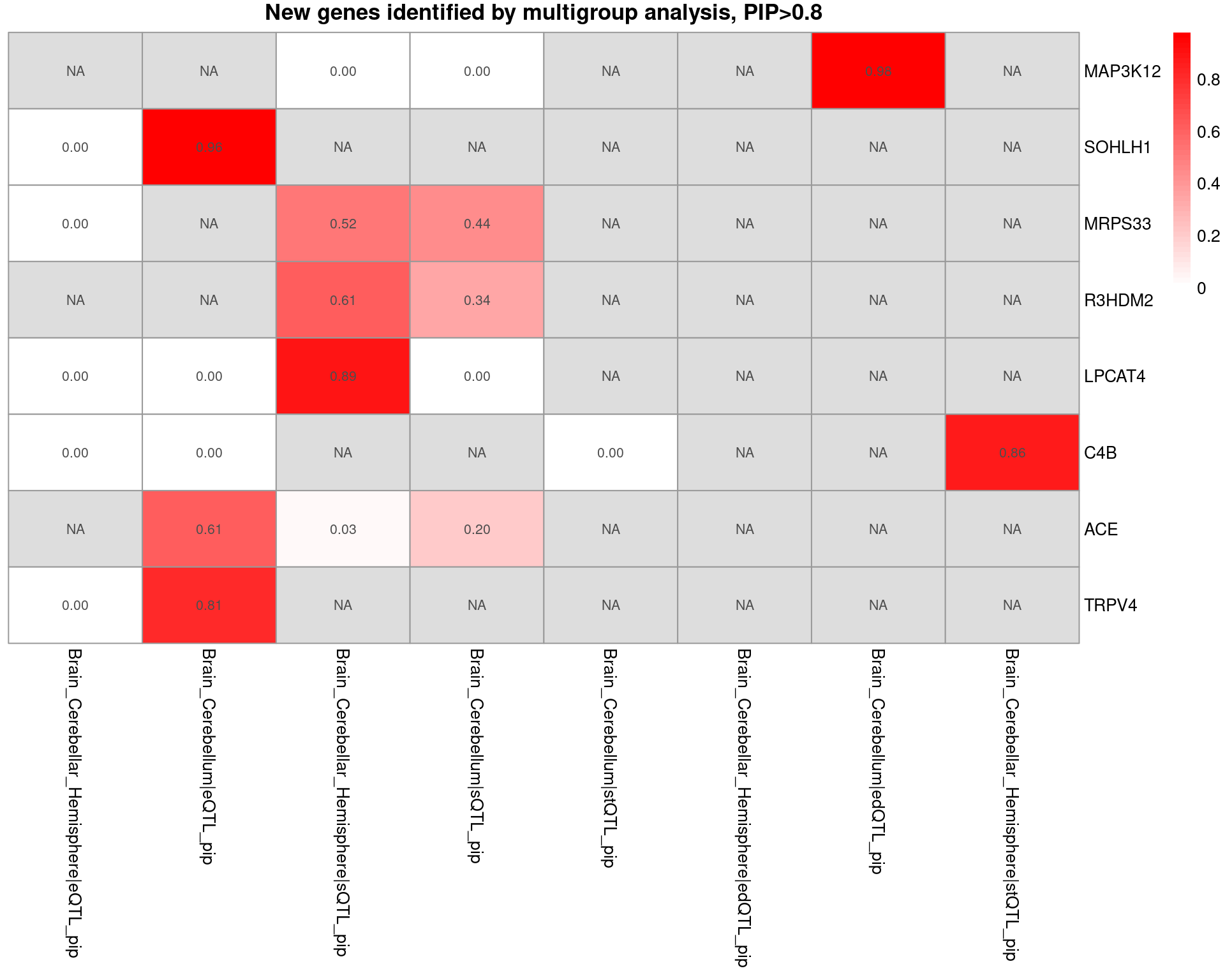
[1] "Unique genes from multigroup: MAP3K12, SOHLH1, MRPS33, R3HDM2, LPCAT4, C4B, ACE, TRPV4"

ASD-ieu-a-1185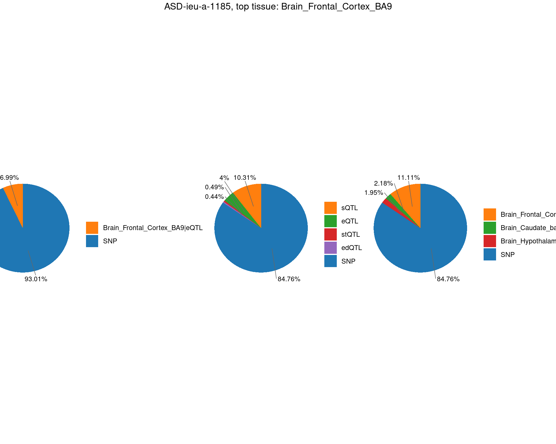
TableGrob (2 x 3) "arrange": 4 grobs
  z     cells    name                 grob
1 1 (2-2,1-1) arrange       gtable[layout]
2 2 (2-2,2-2) arrange       gtable[layout]
3 3 (2-2,3-3) arrange       gtable[layout]
4 4 (1-1,1-3) arrange text[GRID.text.3514]
$plot
$single_genes_unique
character(0)
[1] "Unique genes from multigroup: "
BIP-ieu-b-5110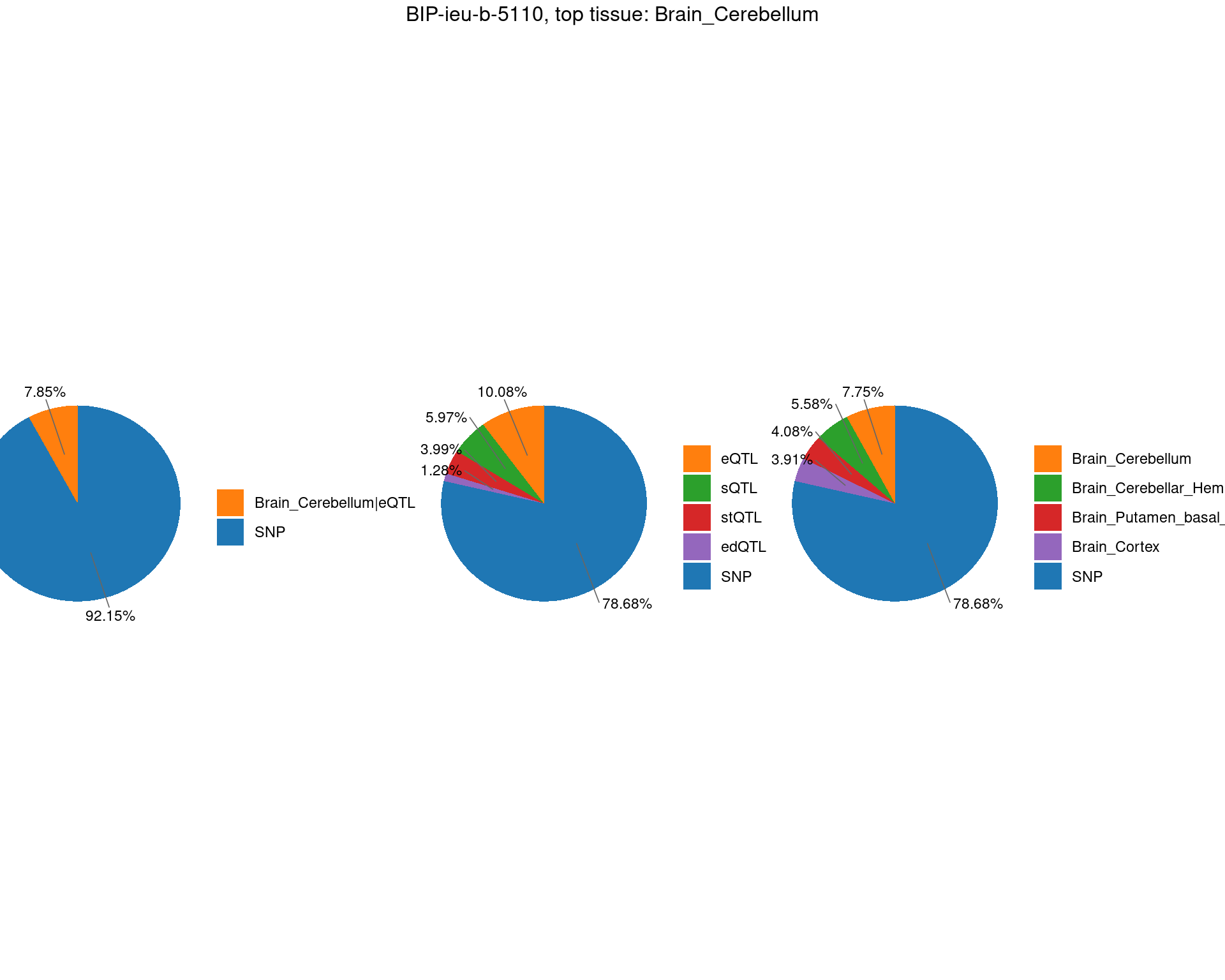
TableGrob (2 x 3) "arrange": 4 grobs
  z     cells    name                 grob
1 1 (2-2,1-1) arrange       gtable[layout]
2 2 (2-2,2-2) arrange       gtable[layout]
3 3 (2-2,3-3) arrange       gtable[layout]
4 4 (1-1,1-3) arrange text[GRID.text.3704]
$plot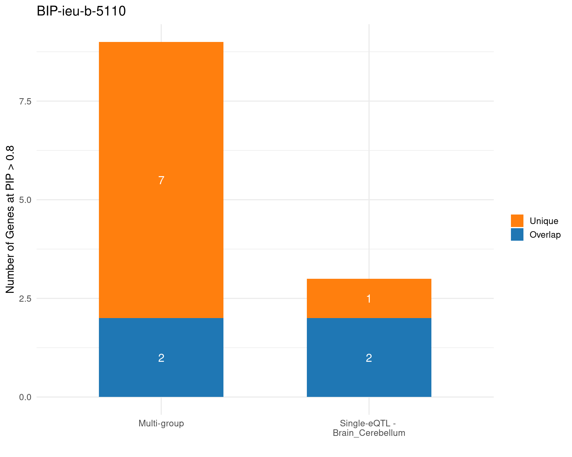
$single_genes_unique
[1] "ZDHHC2"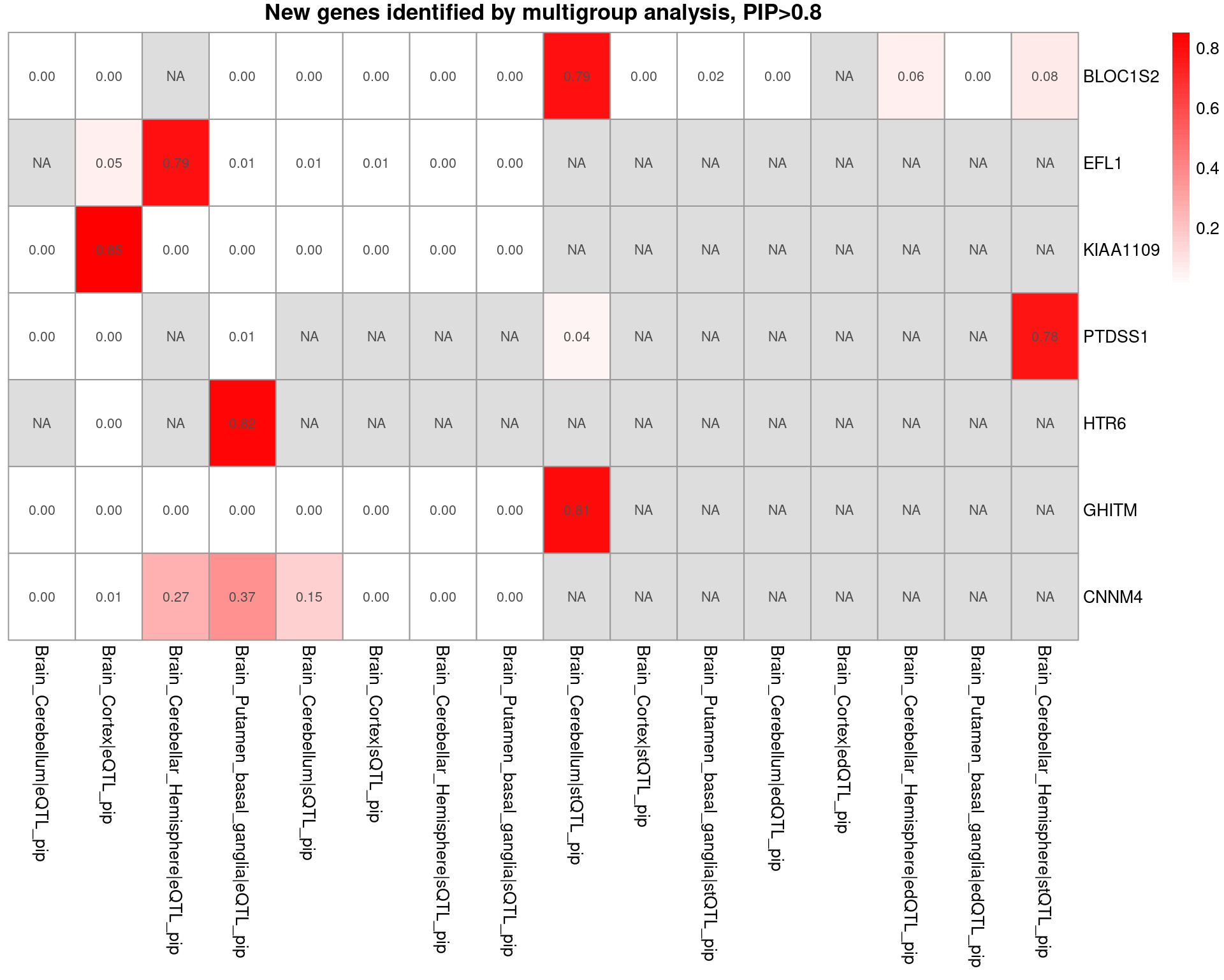
[1] "Unique genes from multigroup: BLOC1S2, EFL1, KIAA1109, PTDSS1, HTR6, GHITM, CNNM4"

MDD-ieu-b-102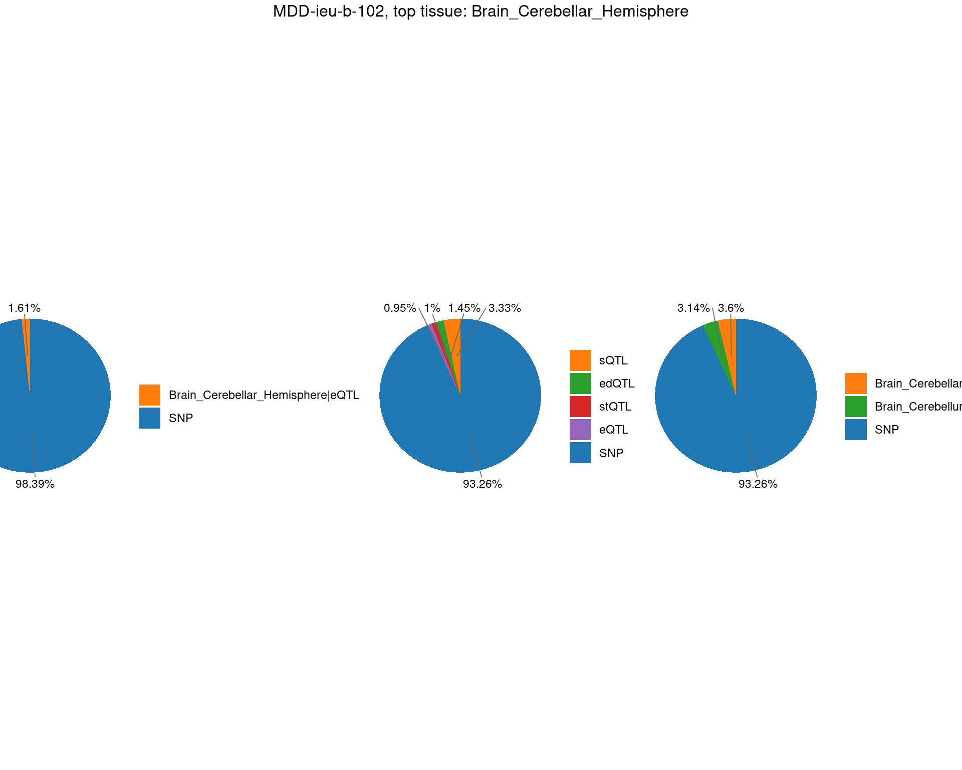
TableGrob (2 x 3) "arrange": 4 grobs
  z     cells    name                 grob
1 1 (2-2,1-1) arrange       gtable[layout]
2 2 (2-2,2-2) arrange       gtable[layout]
3 3 (2-2,3-3) arrange       gtable[layout]
4 4 (1-1,1-3) arrange text[GRID.text.3901]
$plot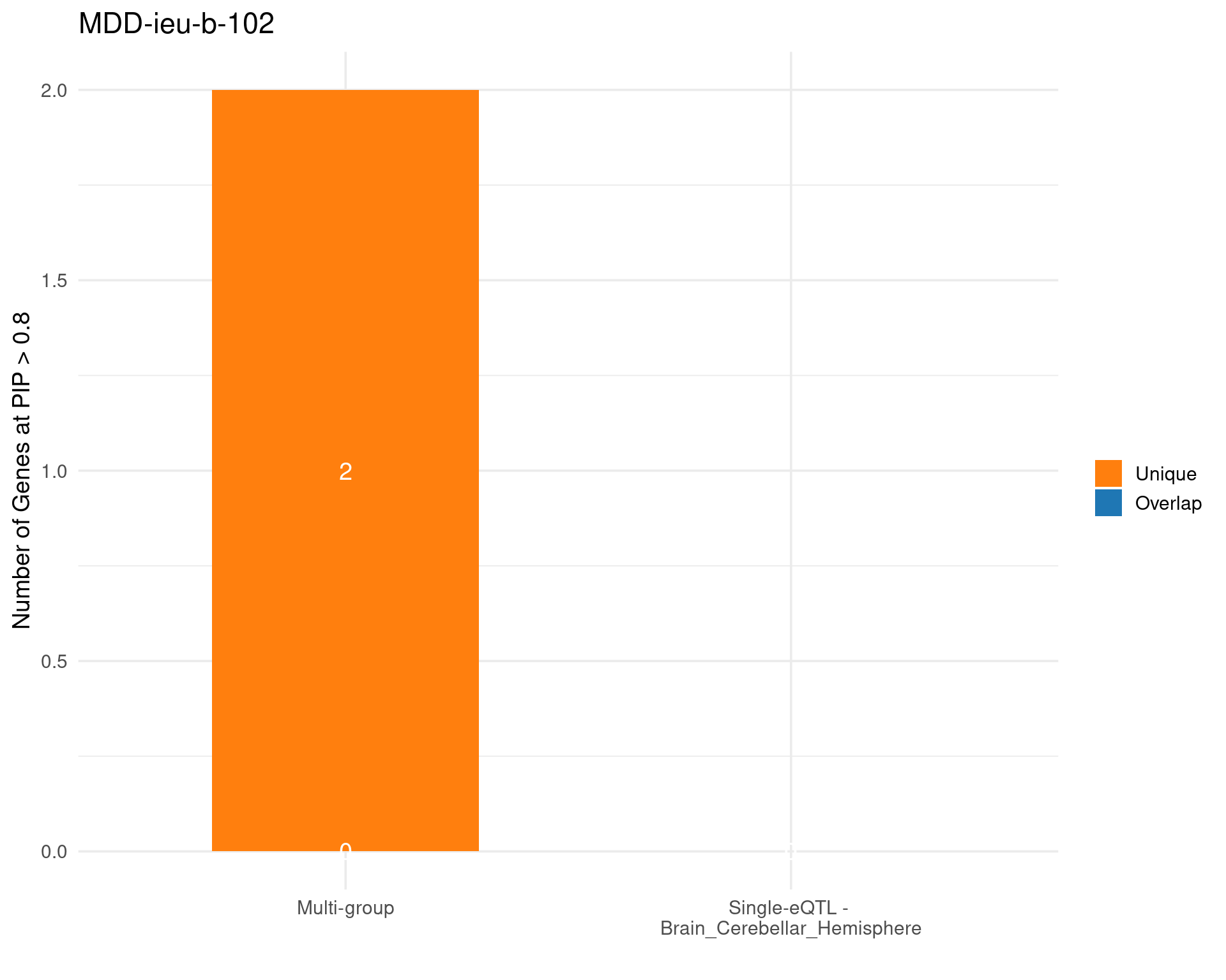
$single_genes_unique
character(0)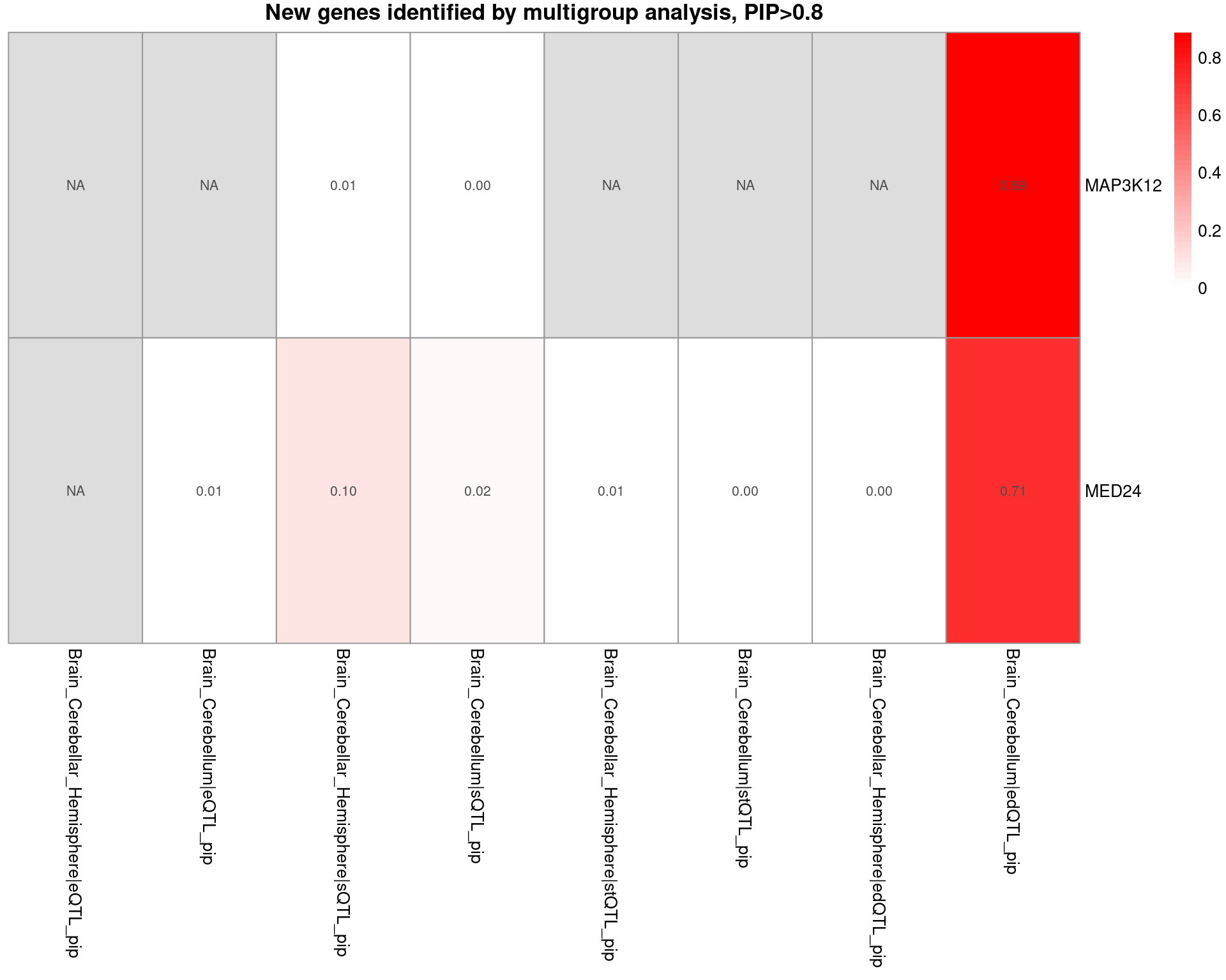
[1] "Unique genes from multigroup: MAP3K12, MED24"

PD-ieu-b-7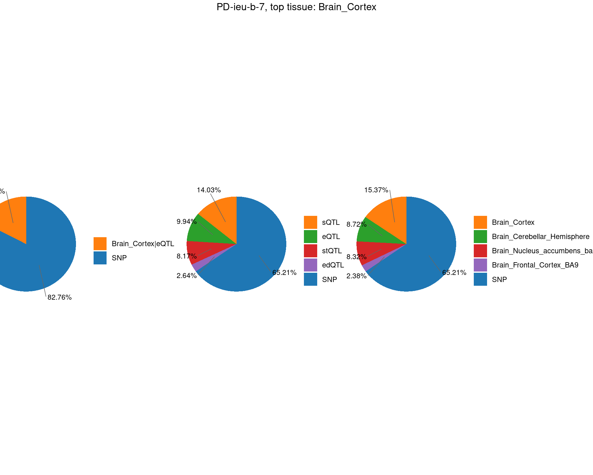
TableGrob (2 x 3) "arrange": 4 grobs
  z     cells    name                 grob
1 1 (2-2,1-1) arrange       gtable[layout]
2 2 (2-2,2-2) arrange       gtable[layout]
3 3 (2-2,3-3) arrange       gtable[layout]
4 4 (1-1,1-3) arrange text[GRID.text.4104]
$plot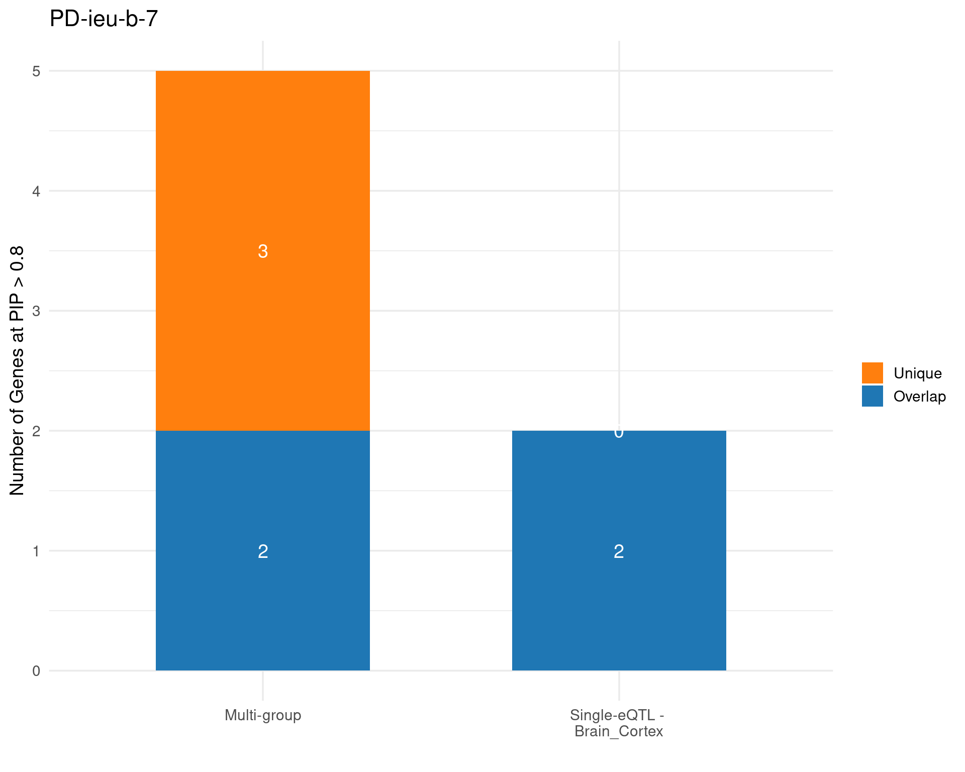
$single_genes_unique
character(0)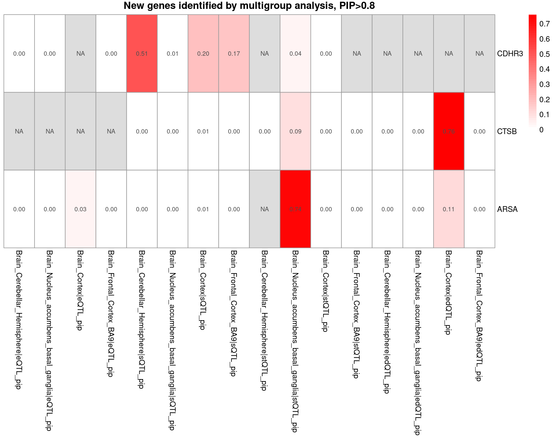
[1] "Unique genes from multigroup: CDHR3, CTSB, ARSA"

ADHD-ieu-a-1183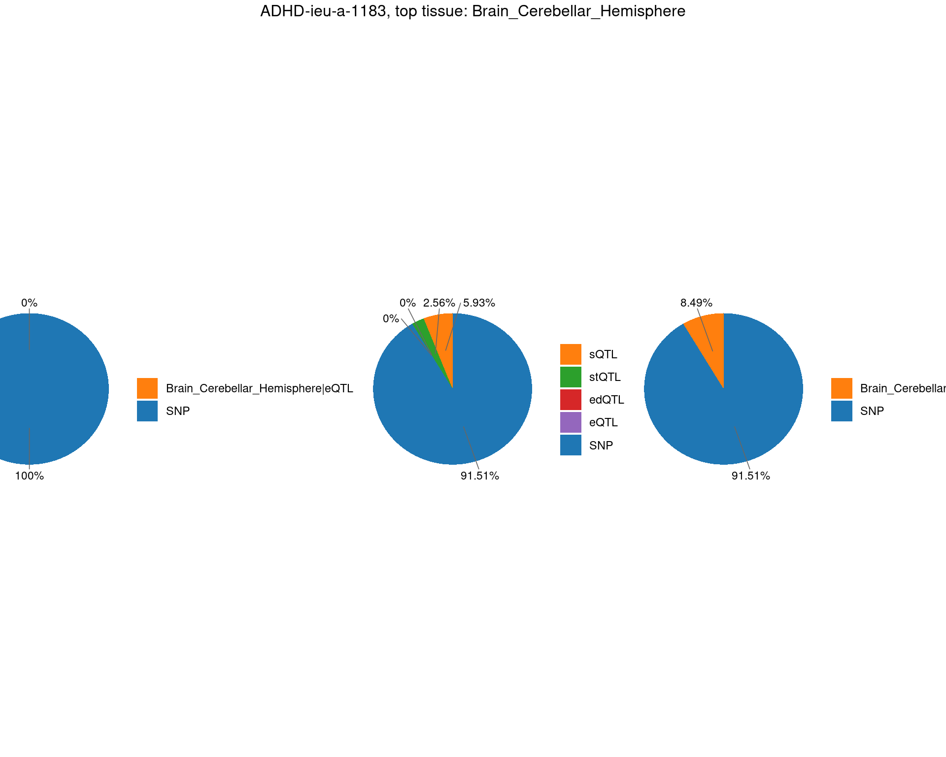
TableGrob (2 x 3) "arrange": 4 grobs
  z     cells    name                 grob
1 1 (2-2,1-1) arrange       gtable[layout]
2 2 (2-2,2-2) arrange       gtable[layout]
3 3 (2-2,3-3) arrange       gtable[layout]
4 4 (1-1,1-3) arrange text[GRID.text.4297]
$plot
$single_genes_unique
character(0)
[1] "Unique genes from multigroup: "
NS-ukb-a-230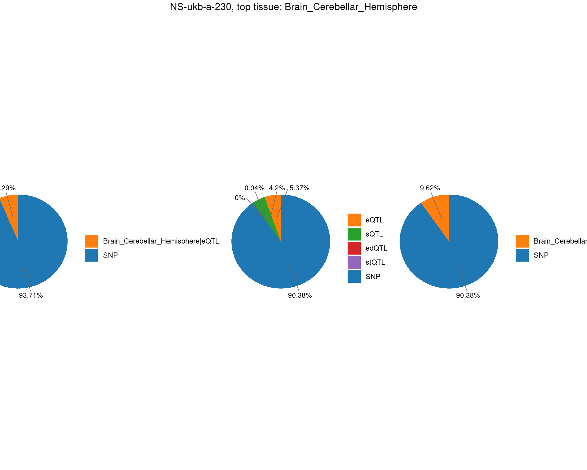
TableGrob (2 x 3) "arrange": 4 grobs
  z     cells    name                 grob
1 1 (2-2,1-1) arrange       gtable[layout]
2 2 (2-2,2-2) arrange       gtable[layout]
3 3 (2-2,3-3) arrange       gtable[layout]
4 4 (1-1,1-3) arrange text[GRID.text.4473]
$plot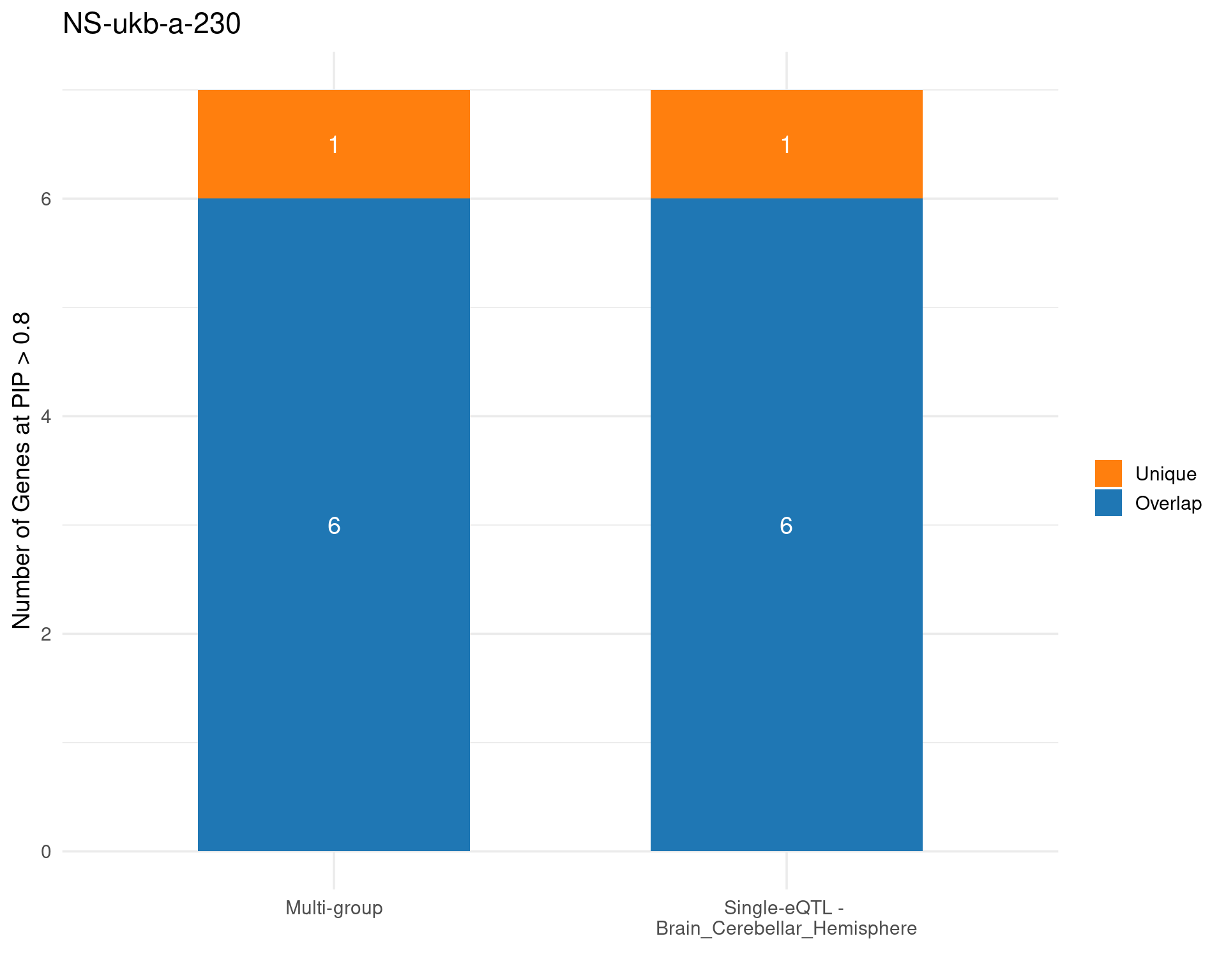
$single_genes_unique
[1] "THRA"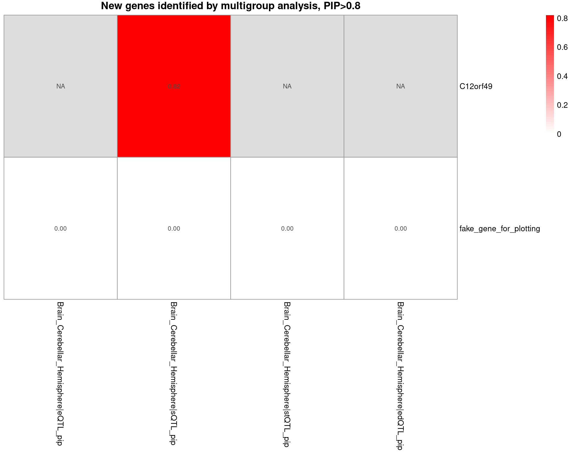
[1] "Unique genes from multigroup: C12orf49"
sessionInfo()R version 4.2.0 (2022-04-22)
Platform: x86_64-pc-linux-gnu (64-bit)
Running under: CentOS Linux 7 (Core)
Matrix products: default
BLAS/LAPACK: /software/openblas-0.3.13-el7-x86_64/lib/libopenblas_haswellp-r0.3.13.so
locale:
[1] C
attached base packages:
[1] grid stats graphics grDevices utils datasets methods
[8] base
other attached packages:
[1] egg_0.4.5 gridExtra_2.3 ggrepel_0.9.1 dplyr_1.1.4
[5] ggplot2_3.5.1 pheatmap_1.0.12 ctwas_0.5.19
loaded via a namespace (and not attached):
[1] colorspace_2.0-3 rjson_0.2.21
[3] ellipsis_0.3.2 rprojroot_2.0.3
[5] XVector_0.36.0 locuszoomr_0.2.1
[7] GenomicRanges_1.48.0 base64enc_0.1-3
[9] fs_1.5.2 rstudioapi_0.13
[11] farver_2.1.0 bit64_4.0.5
[13] AnnotationDbi_1.58.0 fansi_1.0.3
[15] xml2_1.3.3 codetools_0.2-18
[17] logging_0.10-108 cachem_1.0.6
[19] knitr_1.39 jsonlite_1.8.0
[21] workflowr_1.7.0 Rsamtools_2.12.0
[23] dbplyr_2.1.1 png_0.1-7
[25] readr_2.1.2 compiler_4.2.0
[27] httr_1.4.3 assertthat_0.2.1
[29] Matrix_1.5-3 fastmap_1.1.0
[31] lazyeval_0.2.2 cli_3.6.1
[33] later_1.3.0 htmltools_0.5.2
[35] prettyunits_1.1.1 tools_4.2.0
[37] gtable_0.3.0 glue_1.6.2
[39] GenomeInfoDbData_1.2.8 rappdirs_0.3.3
[41] Rcpp_1.0.12 Biobase_2.56.0
[43] jquerylib_0.1.4 vctrs_0.6.5
[45] Biostrings_2.64.0 rtracklayer_1.56.0
[47] xfun_0.41 stringr_1.5.1
[49] irlba_2.3.5 lifecycle_1.0.4
[51] restfulr_0.0.14 ensembldb_2.20.2
[53] XML_3.99-0.14 zlibbioc_1.42.0
[55] zoo_1.8-10 scales_1.3.0
[57] gggrid_0.2-0 hms_1.1.1
[59] promises_1.2.0.1 MatrixGenerics_1.8.0
[61] ProtGenerics_1.28.0 parallel_4.2.0
[63] SummarizedExperiment_1.26.1 RColorBrewer_1.1-3
[65] AnnotationFilter_1.20.0 LDlinkR_1.2.3
[67] yaml_2.3.5 curl_4.3.2
[69] memoise_2.0.1 sass_0.4.1
[71] biomaRt_2.54.1 stringi_1.7.6
[73] RSQLite_2.3.1 highr_0.9
[75] S4Vectors_0.34.0 BiocIO_1.6.0
[77] GenomicFeatures_1.48.3 BiocGenerics_0.42.0
[79] filelock_1.0.2 BiocParallel_1.30.3
[81] repr_1.1.4 GenomeInfoDb_1.39.9
[83] rlang_1.1.2 pkgconfig_2.0.3
[85] matrixStats_0.62.0 bitops_1.0-7
[87] evaluate_0.15 lattice_0.20-45
[89] purrr_1.0.2 labeling_0.4.2
[91] GenomicAlignments_1.32.0 htmlwidgets_1.5.4
[93] cowplot_1.1.1 bit_4.0.4
[95] tidyselect_1.2.0 magrittr_2.0.3
[97] AMR_2.1.1 R6_2.5.1
[99] IRanges_2.30.0 generics_0.1.2
[101] DelayedArray_0.22.0 DBI_1.2.2
[103] withr_2.5.0 pgenlibr_0.3.3
[105] pillar_1.9.0 KEGGREST_1.36.3
[107] RCurl_1.98-1.7 mixsqp_0.3-43
[109] tibble_3.2.1 crayon_1.5.1
[111] utf8_1.2.2 BiocFileCache_2.4.0
[113] plotly_4.10.0 tzdb_0.4.0
[115] rmarkdown_2.25 progress_1.2.2
[117] data.table_1.14.2 blob_1.2.3
[119] git2r_0.30.1 digest_0.6.29
[121] tidyr_1.3.0 httpuv_1.6.5
[123] stats4_4.2.0 munsell_0.5.0
[125] viridisLite_0.4.0 skimr_2.1.4
[127] bslib_0.3.1