Multi group analysis: 6 traits, 5 tissues, eQTL + sQTL + apaQTL – Compute UKBB LD
XSun
2024-05-27
Last updated: 2024-06-28
Checks: 6 1
Knit directory: multigroup_ctwas_analysis/
This reproducible R Markdown analysis was created with workflowr (version 1.7.0). The Checks tab describes the reproducibility checks that were applied when the results were created. The Past versions tab lists the development history.
The R Markdown file has unstaged changes. To know which version of
the R Markdown file created these results, you’ll want to first commit
it to the Git repo. If you’re still working on the analysis, you can
ignore this warning. When you’re finished, you can run
wflow_publish to commit the R Markdown file and build the
HTML.
Great job! The global environment was empty. Objects defined in the global environment can affect the analysis in your R Markdown file in unknown ways. For reproduciblity it’s best to always run the code in an empty environment.
The command set.seed(20231112) was run prior to running
the code in the R Markdown file. Setting a seed ensures that any results
that rely on randomness, e.g. subsampling or permutations, are
reproducible.
Great job! Recording the operating system, R version, and package versions is critical for reproducibility.
Nice! There were no cached chunks for this analysis, so you can be confident that you successfully produced the results during this run.
Great job! Using relative paths to the files within your workflowr project makes it easier to run your code on other machines.
Great! You are using Git for version control. Tracking code development and connecting the code version to the results is critical for reproducibility.
The results in this page were generated with repository version c48ee25. See the Past versions tab to see a history of the changes made to the R Markdown and HTML files.
Note that you need to be careful to ensure that all relevant files for
the analysis have been committed to Git prior to generating the results
(you can use wflow_publish or
wflow_git_commit). workflowr only checks the R Markdown
file, but you know if there are other scripts or data files that it
depends on. Below is the status of the Git repository when the results
were generated:
Ignored files:
    Ignored:    .Rhistory
    Ignored:    results/

Unstaged changes:
    Modified:   analysis/multi_group_6traits_15weights_ukbb.Rmd
Note that any generated files, e.g. HTML, png, CSS, etc., are not included in this status report because it is ok for generated content to have uncommitted changes.
These are the previous versions of the repository in which changes were
made to the R Markdown
(analysis/multi_group_6traits_15weights_ukbb.Rmd) and HTML
(docs/multi_group_6traits_15weights_ukbb.html) files. If
you’ve configured a remote Git repository (see
?wflow_git_remote), click on the hyperlinks in the table
below to view the files as they were in that past version.
| File | Version | Author | Date | Message |
|---|---|---|---|---|
| Rmd | 9e83189 | XSun | 2024-06-13 | update |
| html | 9e83189 | XSun | 2024-06-13 | update |
| Rmd | f82f6b4 | XSun | 2024-06-11 | update |
| html | f82f6b4 | XSun | 2024-06-11 | update |
| Rmd | 44f18ae | XSun | 2024-06-02 | update |
| html | 44f18ae | XSun | 2024-06-02 | update |
| Rmd | b7b6005 | XSun | 2024-05-31 | update |
| html | b7b6005 | XSun | 2024-05-31 | update |
| Rmd | b1914dd | XSun | 2024-05-31 | update |
| html | b1914dd | XSun | 2024-05-31 | update |
| Rmd | 163c010 | XSun | 2024-05-31 | update |
| html | 163c010 | XSun | 2024-05-31 | update |
| Rmd | 2b980bb | XSun | 2024-05-30 | update |
| html | 2b980bb | XSun | 2024-05-30 | update |
Overview
Tissues
The independent tissues are selected by single tissue analysis
Omics
eQTL, sQTL weights are from GTEx PredictDB
apaQTL wetights are from https://www.nature.com/articles/s41467-024-46064-7#Sec2. Top 10 SNPs with largest abs(weights) were selected after harmonization
Settings
- Weight processing:
PredictDB:
- drop_strand_ambig = TRUE,
- scale_by_ld_variance = TRUE,
- load_predictdb_LD = F,
FUSION:
- method_FUSION = “enet”,
- fusion_top_n_snps = 10,
- drop_strand_ambig = TRUE,
- scale_by_ld_variance = F,
- load_predictdb_LD = F,
- Parameter estimation and fine-mapping
- niter_prefit = 5,
- niter = 60,
- L = 3,
- group_prior_var_structure = “shared_type”,
- maxSNP = 20000,
- min_nonSNP_PIP = 0.5,
- Memory requested
- cpus-per-task=2
- mem=200G
100G 2core got killed
Results
Results from multi-group analysis
The results are summarized by
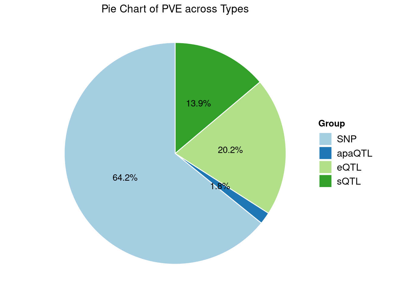
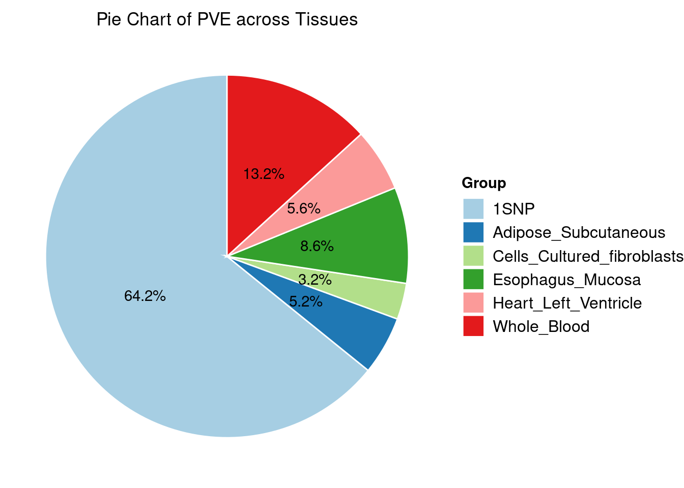
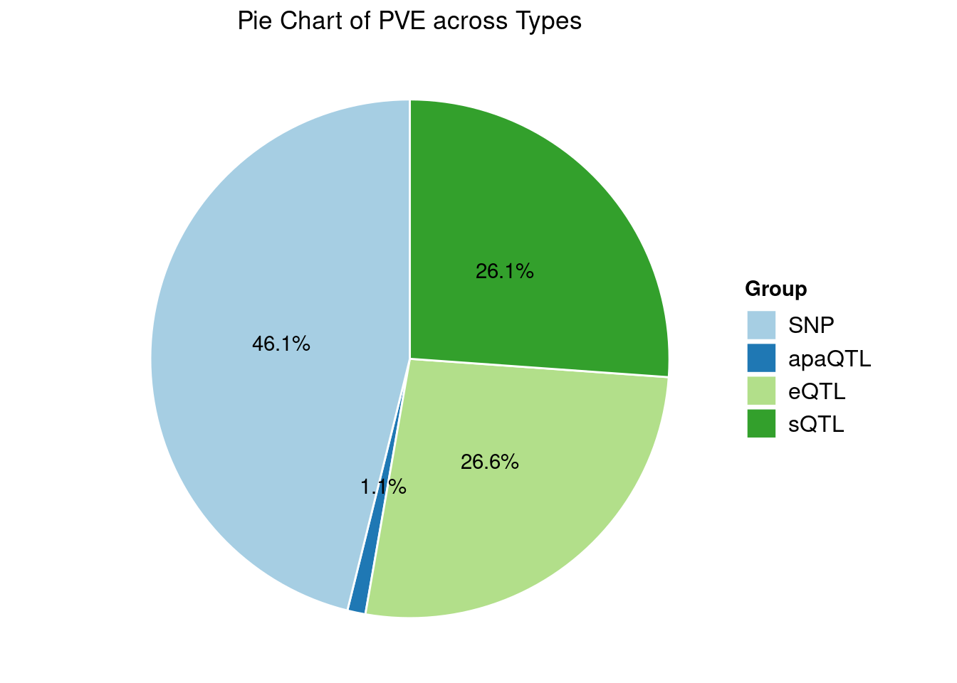
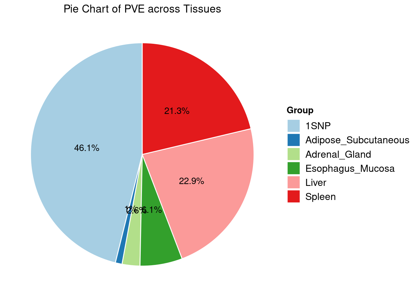
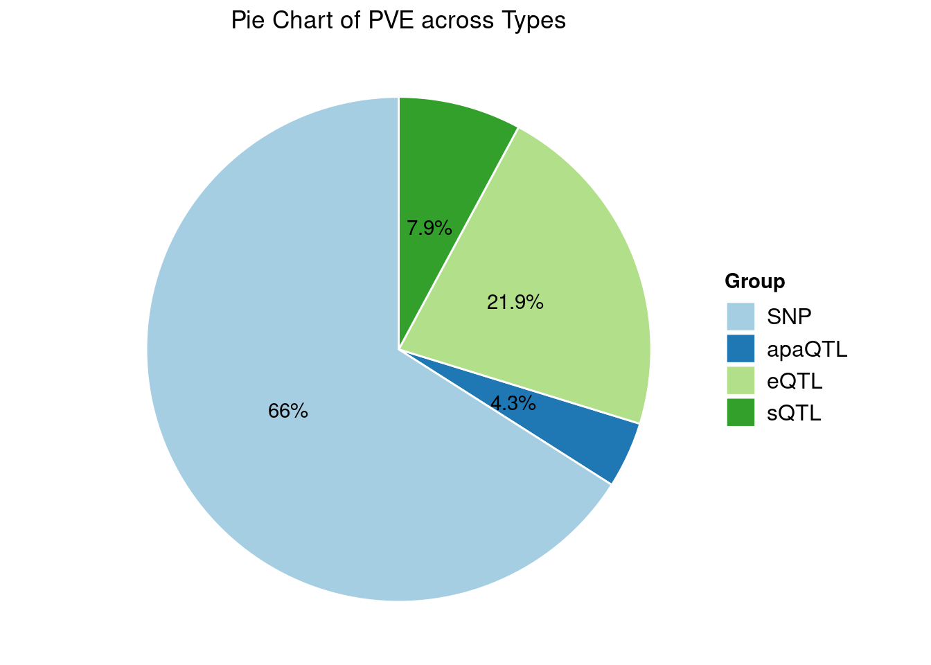
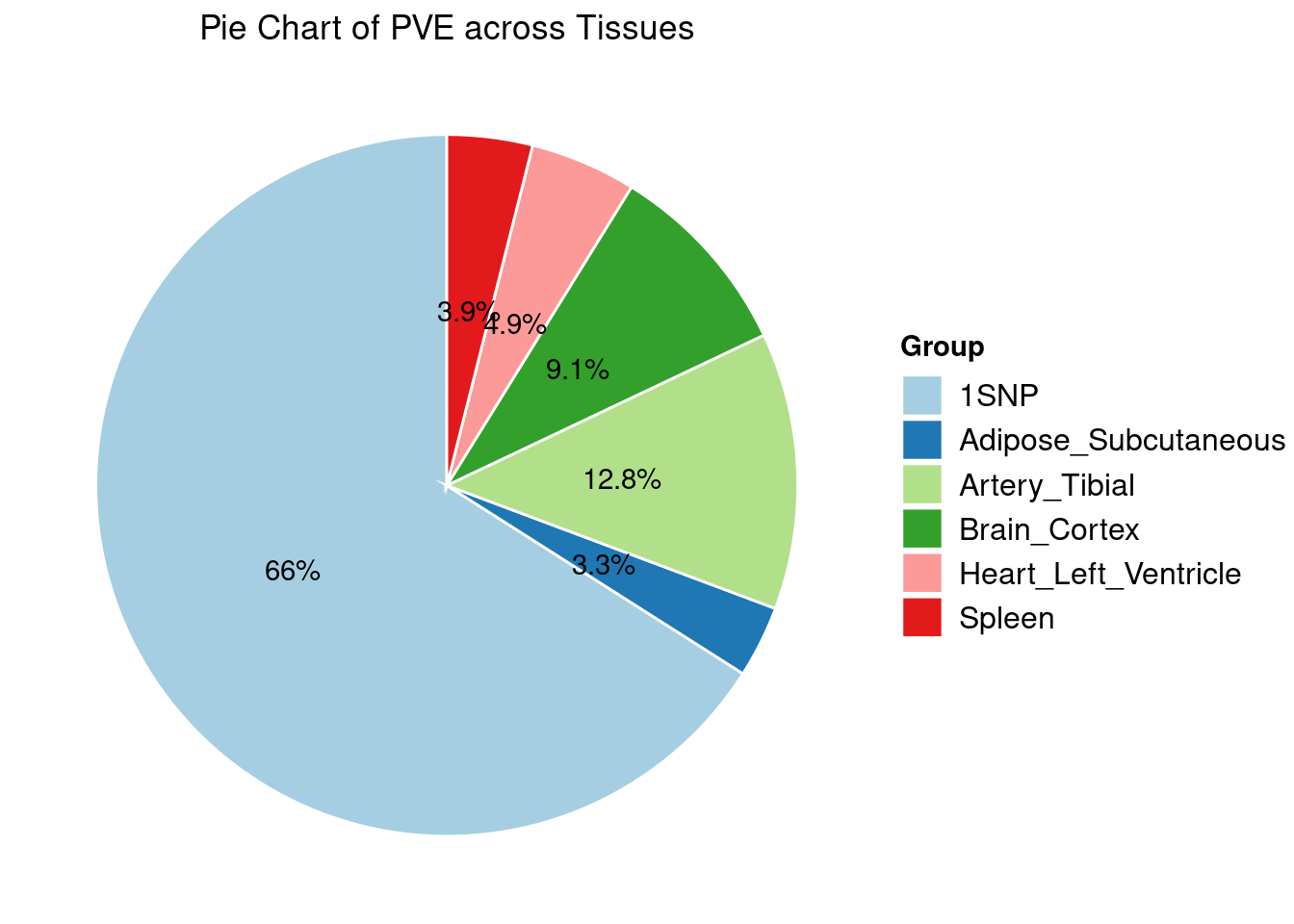
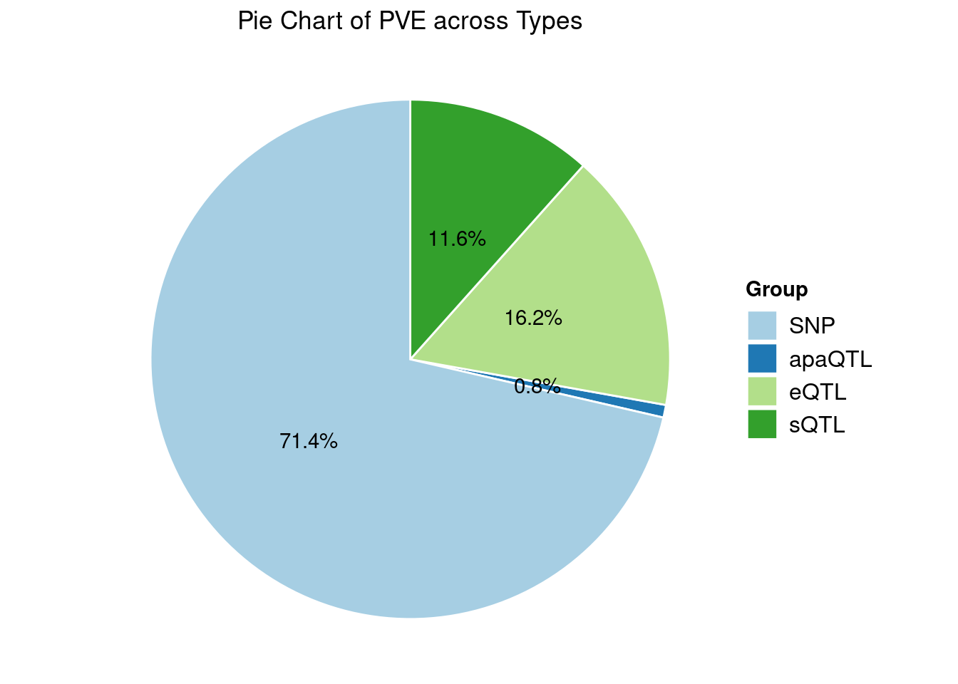
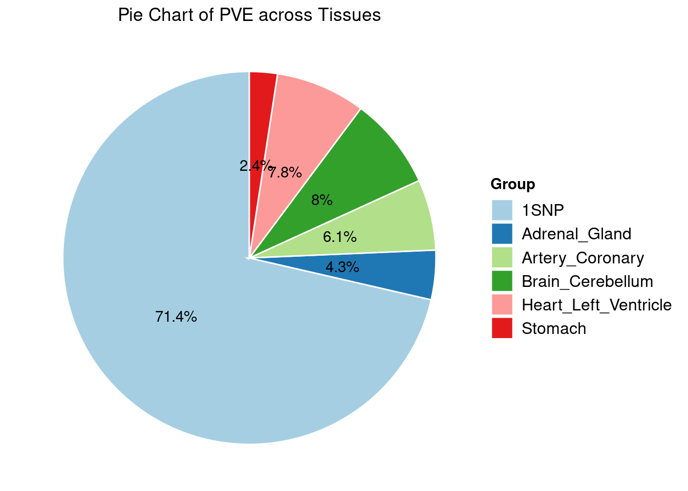
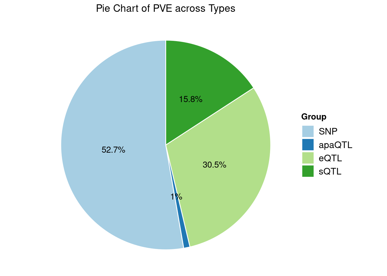
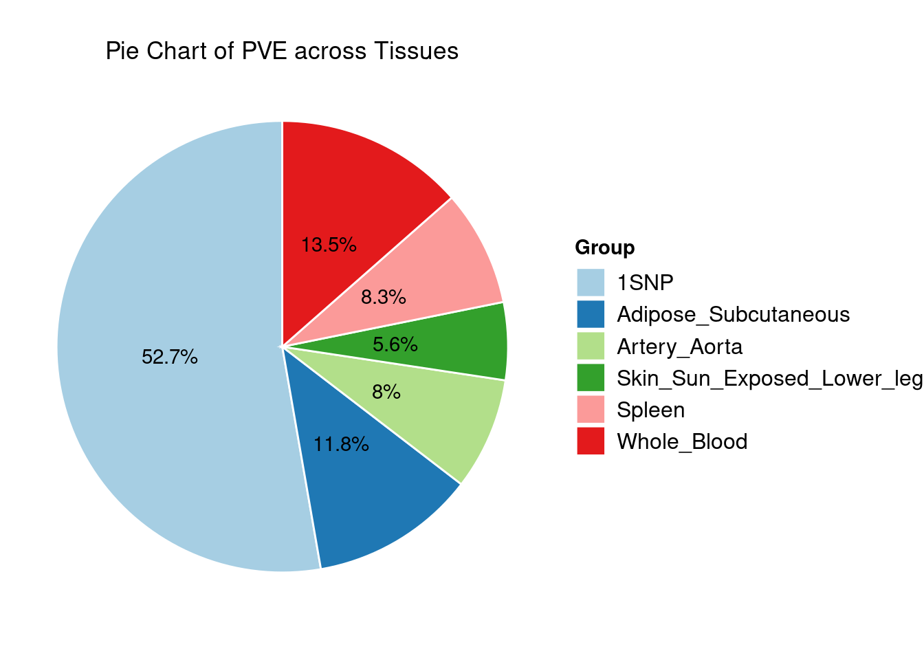
Heritability contribution by contexts: we aggregate the PVE values by omics and tissues, making it easier to understand the distribution of PVE across different genetic contexts.
Combined PIP by omics: we aggregate the Susie PIPs by omics
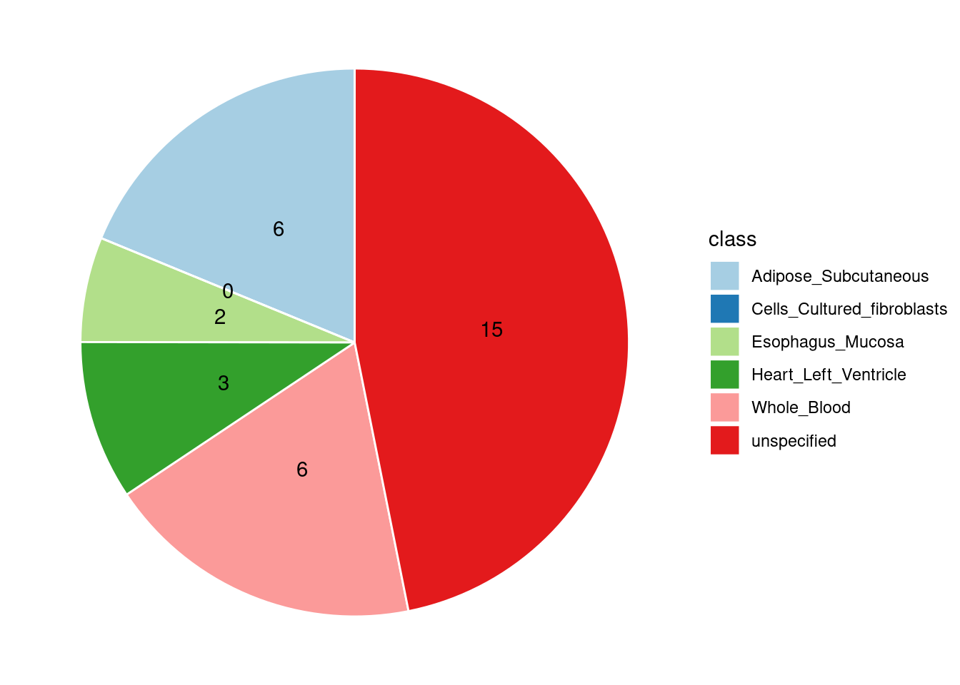
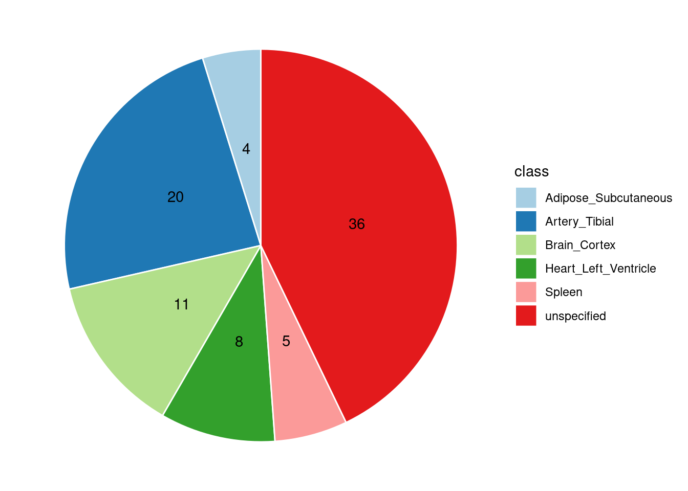
Combined PIP by contexts: we aggregate the Susie PIPs by tissues, making it easier to understand the distribution of PIP across different genetic contexts.
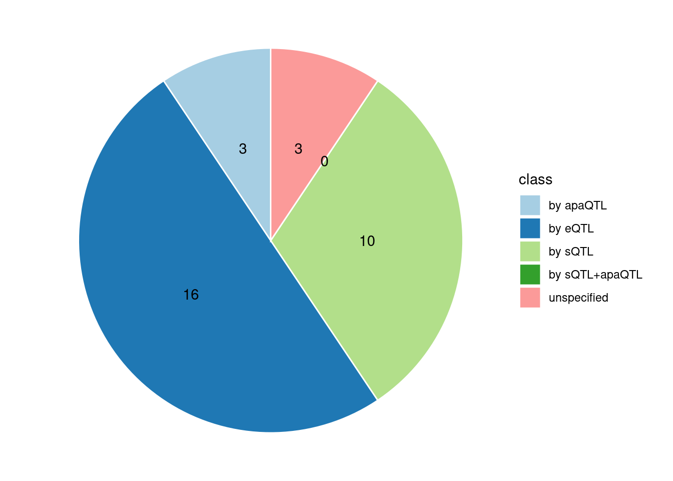
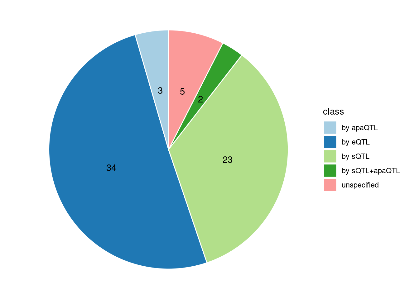
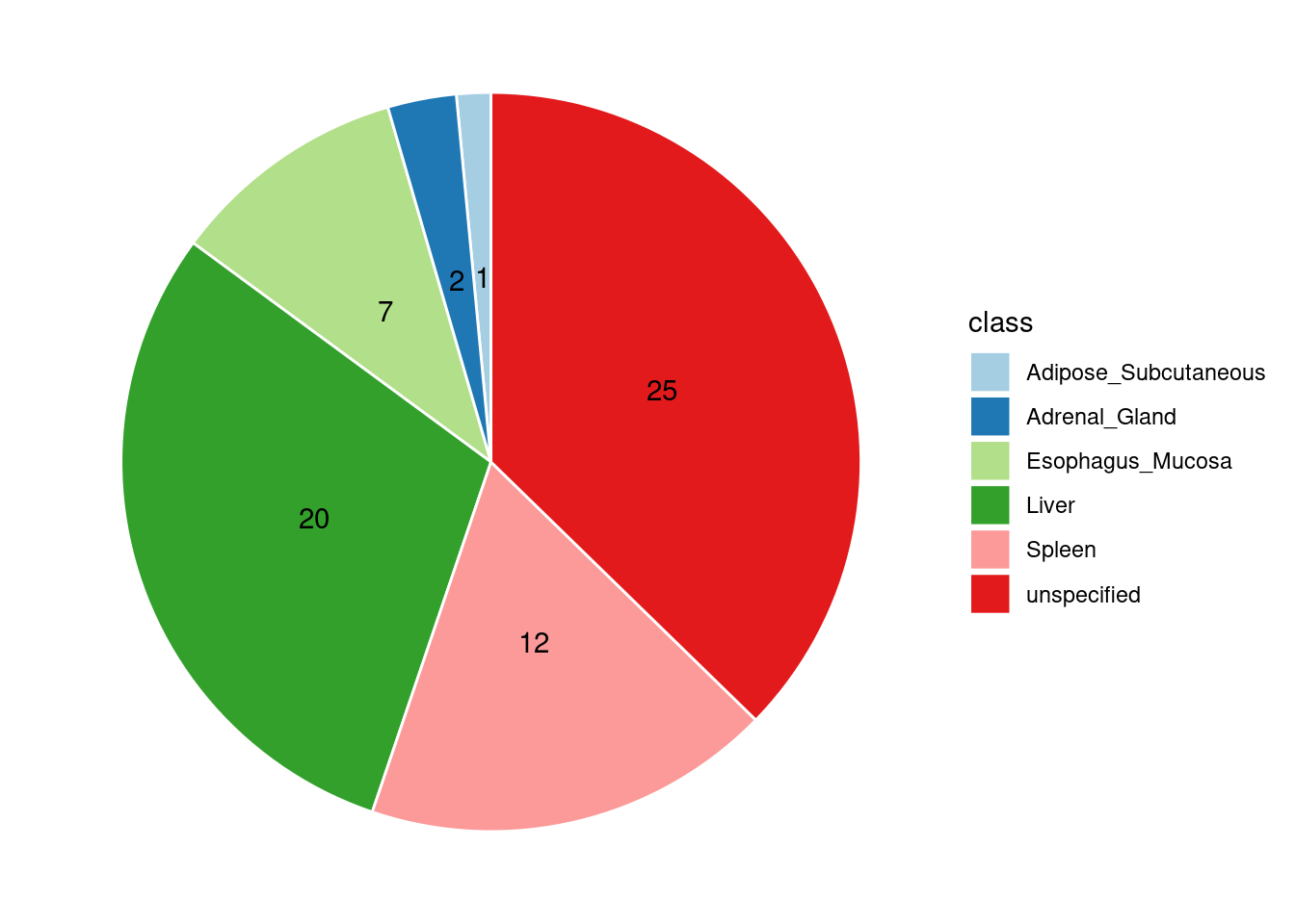
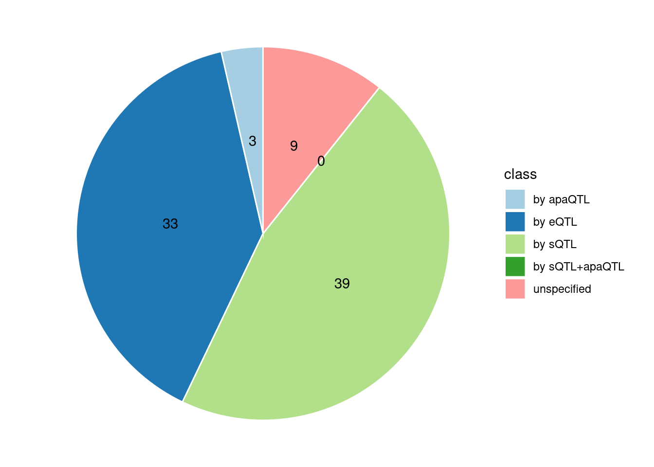
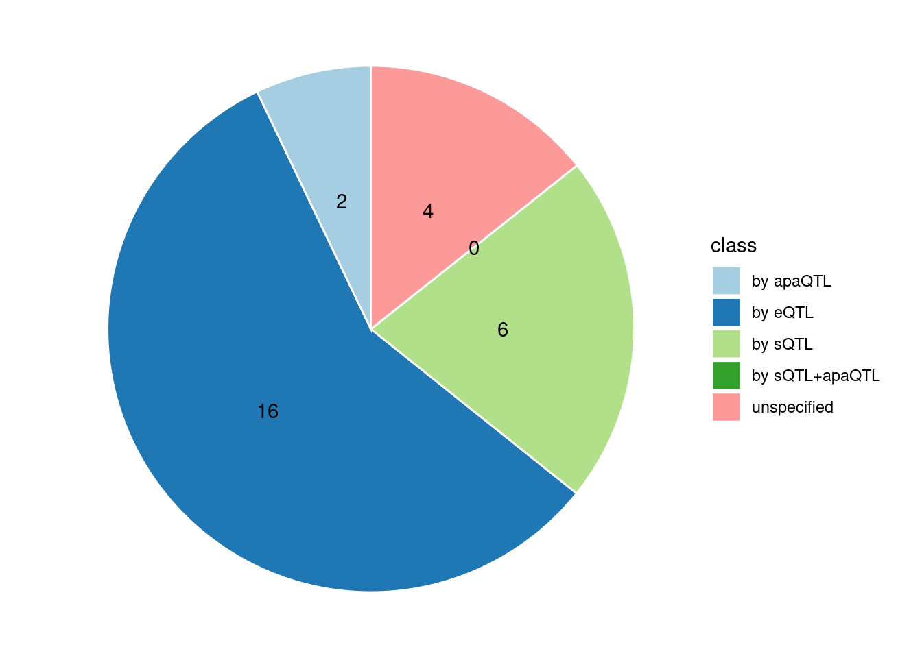
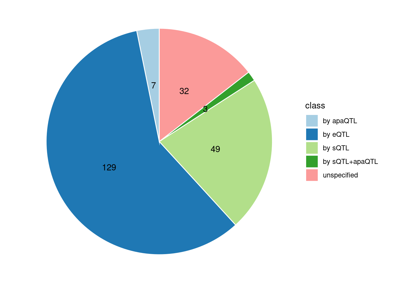
Specific molecular traits of top genes: we creates a pie chart to visualize the proportion of genes classified into different categories based on their PIPs contributed by each genetics contexts. The categories are based on the proportion of each QTL type relative to the combined PIP value:
- by eQTL: Number of genes where the ratio of eQTL to combined PIP is greater than 0.8.
- by sQTL: Number of genes where the ratio of sQTL to combined PIP is greater than 0.8.
- by apaQTL: Number of genes where the ratio of apaQTL to combined PIP is greater than 0.8.
- by sQTL+apaQTL: Number of genes where the combined ratio of apaQTL and sQTL to combined PIP is greater than 0.8, but neither apaQTL nor sQTL individually exceed 0.8.
- unspecified: Number of genes not classified into any of the above categories.
Comparing with single group eQTL results
Please not that the ealier single group eQTL analyses were performed under L=5 but the current analyses were under L=3
We compared number of significant genes, overlapping genes and the changes in PVE for eQTLs across five tissues reported by single eQTL analysi
aFib
TO DO
IBD
Results from multi-group analysis
[1] "Adipose_Subcutaneous"       "Esophagus_Mucosa"
[3] "Whole_Blood"                "Heart_Left_Ventricle"
[5] "Cells_Cultured_fibroblasts"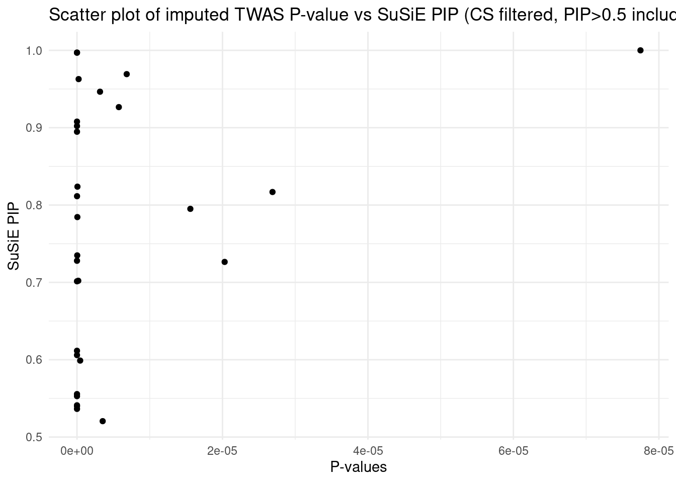
| Version | Author | Date |
|---|---|---|
| 9e83189 | XSun | 2024-06-13 |
Comparing with single group eQTL results
[1] "the top tissues from single group analyses are Cells_Cultured_fibroblasts,Whole_Blood,Adipose_Subcutaneous,Esophagus_Mucosa,Heart_Left_Ventricle"We then looked into Whole_Blood. Please not that the
ealier single group eQTL analyses were performed under L=5
but the current analyses were under L=3.
So we re-ran the single group analysis using L=3 with
for Whole_Blood.
[1] "The number of sig genes reported by single group analysis under L=3 is 10"[1] "The number of overlapped genes is 7"locus zoom plot for the regions containing these genes: https://uchicago.box.com/s/ziv0v006pxwnuprhxbagdfr0cnfk5e23
DT::datatable(df_summary,caption = htmltools::tags$caption( style = 'caption-side: topleft; text-align = left; color:black;','All genes with pip > 0.8 from single group analysis and all genes with combined pip >0.8 from multi group analysis'),options = list(pageLength = 5) )ggplot(df_summary, aes(x = combined_pip_multi_group, y = combined_pip_nonzero_cs_multi_group)) +
geom_point() + # Add points
geom_abline(intercept = 0, slope = 1, color = "red", linetype = "dashed") +
labs(x = "Combined PIP Multi Group (adding up all pips)",
y = "Combined PIP Nonzero CS Multi Group (only pips with non-zero CS added)",
title = "Comparison for combined pip") +
theme_minimal()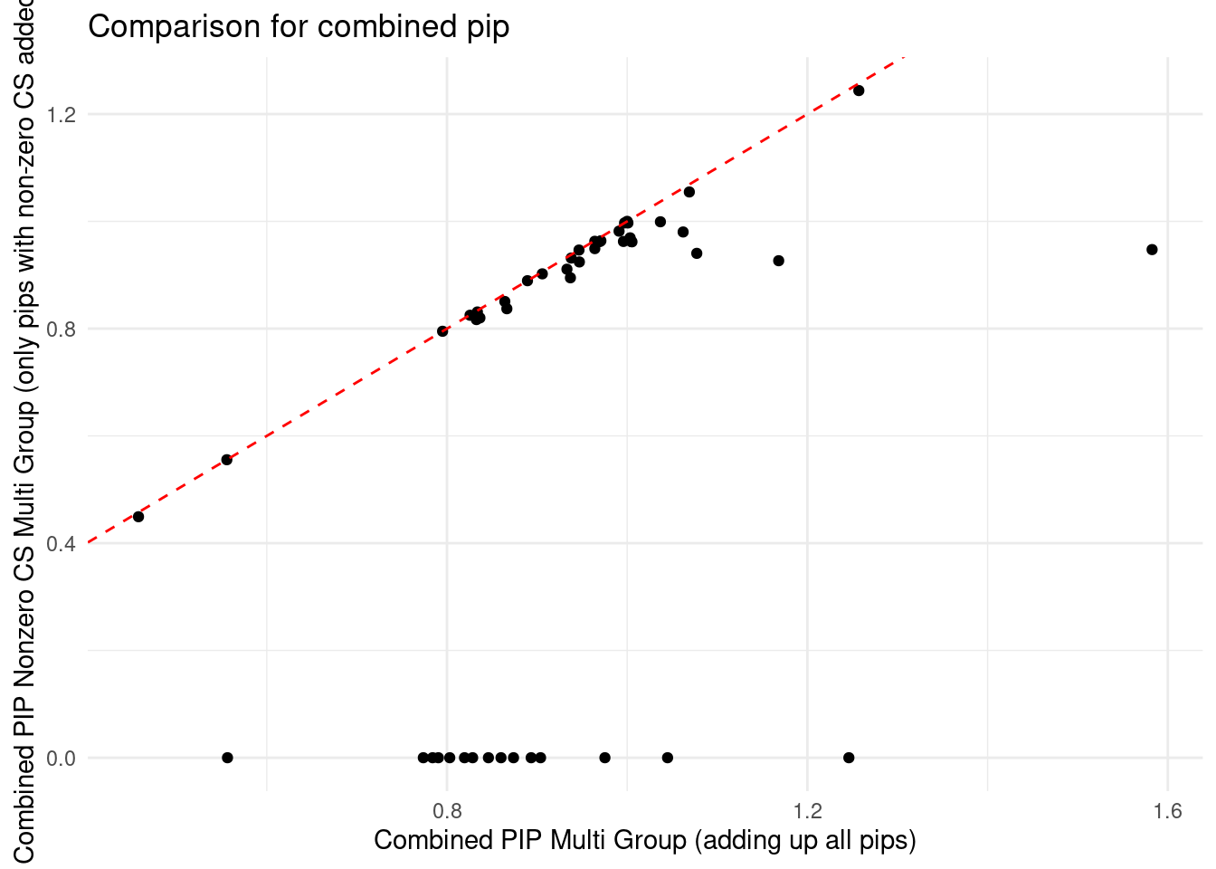
| Version | Author | Date |
|---|---|---|
| 163c010 | XSun | 2024-05-31 |
LDL
Results from multi-group analysis
[1] "Esophagus_Mucosa"     "Liver"                "Spleen"
[4] "Adipose_Subcutaneous" "Adrenal_Gland" 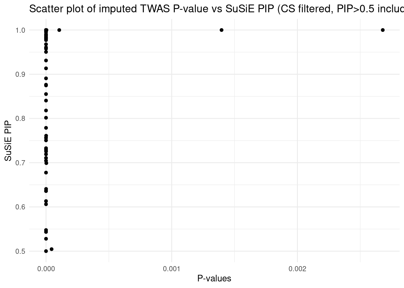
| Version | Author | Date |
|---|---|---|
| 9e83189 | XSun | 2024-06-13 |
Comparing with single group eQTL results
[1] "the top tissues from single group analyses are Liver,Spleen,Adipose_Subcutaneous,Adrenal_Gland,Esophagus_Mucosa"We then looked into Adipose_Subcutaneous. Please not
that the ealier single group eQTL analyses were performed under
L=5 but the current analyses were under
L=3.
So we re-ran the single group analysis using L=3 with
for Adipose_Subcutaneous.
[1] "The number of sig genes reported by single group analysis under L=3 is 16"[1] "The number of overlapped genes is 4"locus zoom plot for the regions containing these genes: https://uchicago.box.com/s/u93gpgil79ybf7akrl1obfkpgkxq5wkn
DT::datatable(df_summary,caption = htmltools::tags$caption( style = 'caption-side: topleft; text-align = left; color:black;','All genes with pip > 0.8 from single group analysis and all genes with combined pip >0.8 from multi group analysis'),options = list(pageLength = 5) )ggplot(df_summary, aes(x = combined_pip_multi_group, y = combined_pip_nonzero_cs_multi_group)) +
geom_point() + # Add points
geom_abline(intercept = 0, slope = 1, color = "red", linetype = "dashed") +
labs(x = "Combined PIP Multi Group (adding up all pips)",
y = "Combined PIP Nonzero CS Multi Group (only pips with non-zero CS added)",
title = "Comparison for combined pip") +
theme_minimal()Warning: Removed 2 rows containing missing values or values outside the scale range
(`geom_point()`).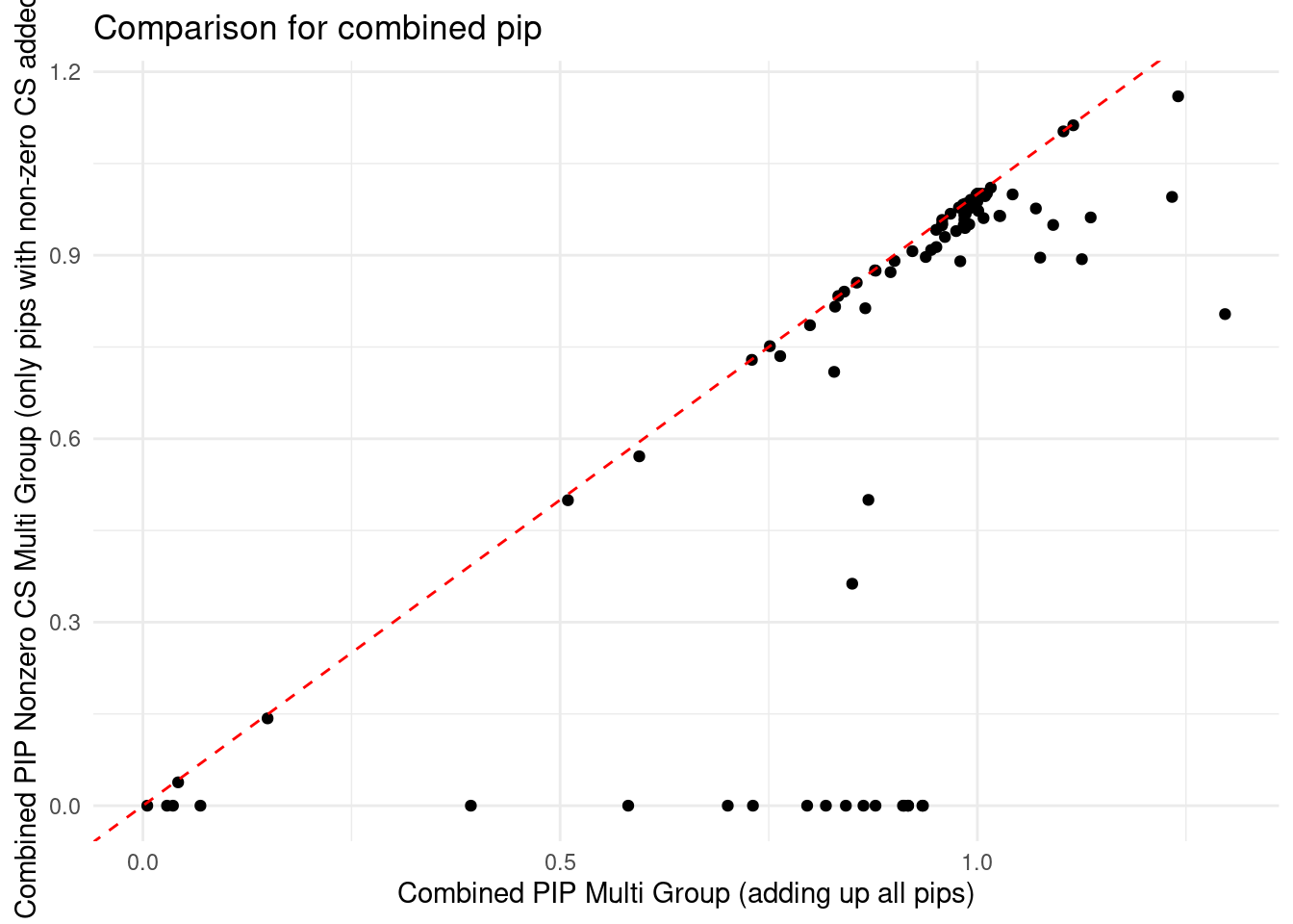
| Version | Author | Date |
|---|---|---|
| 163c010 | XSun | 2024-05-31 |
SBP
Results from multi-group analysis
[1] "Artery_Tibial"        "Heart_Left_Ventricle" "Spleen"
[4] "Brain_Cortex"         "Adipose_Subcutaneous"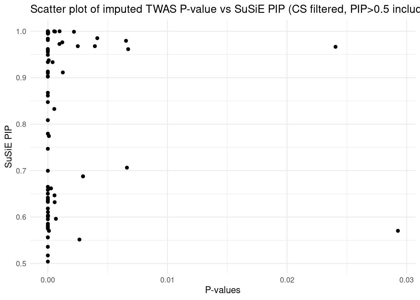
| Version | Author | Date |
|---|---|---|
| 9e83189 | XSun | 2024-06-13 |
plot for this locus https://uchicago.box.com/s/uca02ksxb4hz67lohjpko35nkjhp5pti
We ran regular SuSiE (uniform prior) in a region, and obtain the number of CS from the results. Then we ran fine-mapping step for this region.
By doing these, we have
estimated_L <- readRDS("/project/xinhe/xsun/multi_group_ctwas/5.multi_group_testing/results_preL/SBP-ukb-a-360/SBP-ukb-a-360.estimated_L.RDS")

sprintf("the pre-estimated L is %s", estimated_L["16:2714828-3951195"])
[1] "the pre-estimated L is 1"load("/project/xinhe/xsun/multi_group_ctwas/5.multi_group_testing/analy_results/NAA60.preL.rdata")
DT::datatable(finemap_res_region_multi,caption = htmltools::tags$caption( style = 'caption-side: topleft; text-align = left; color:black;','Updated PIP (run with pre-estimated L)'),options = list(pageLength = 5) )Comparing with single group eQTL results
[1] "the top tissues from single group analyses are Artery_Tibial,Adipose_Subcutaneous,Brain_Cortex,Heart_Left_Ventricle,Spleen"SCZ
Results from multi-group analysis
| Version | Author | Date |
|---|---|---|
| 9e83189 | XSun | 2024-06-13 |
| Version | Author | Date |
|---|---|---|
| 9e83189 | XSun | 2024-06-13 |
| Version | Author | Date |
|---|---|---|
| 9e83189 | XSun | 2024-06-13 |
| Version | Author | Date |
|---|---|---|
| 9e83189 | XSun | 2024-06-13 |
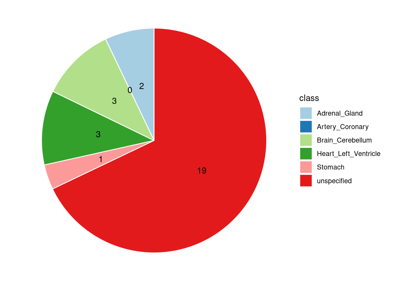
[1] "Heart_Left_Ventricle" "Adrenal_Gland"        "Artery_Coronary"
[4] "Stomach" "Brain_Cerebellum" 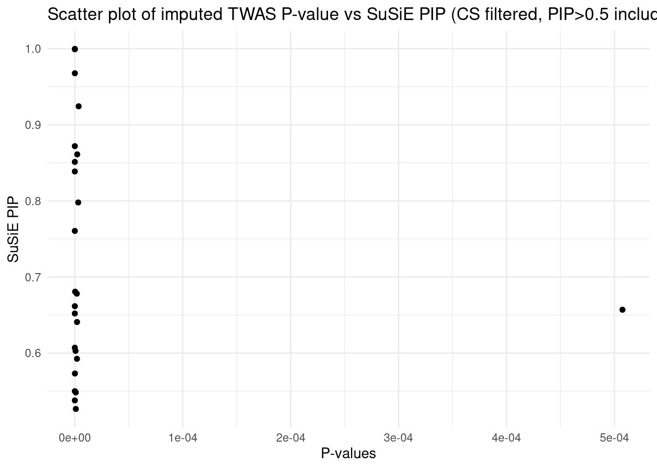
| Version | Author | Date |
|---|---|---|
| 9e83189 | XSun | 2024-06-13 |
Comparing with single group eQTL results
[1] "the top tissues from single group analyses are Heart_Left_Ventricle,Adrenal_Gland,Artery_Coronary,Brain_Cerebellum,Stomach"WBC
Results from multi-group analysis
| Version | Author | Date |
|---|---|---|
| 9e83189 | XSun | 2024-06-13 |
| Version | Author | Date |
|---|---|---|
| 9e83189 | XSun | 2024-06-13 |
| Version | Author | Date |
|---|---|---|
| 9e83189 | XSun | 2024-06-13 |
| Version | Author | Date |
|---|---|---|
| 9e83189 | XSun | 2024-06-13 |
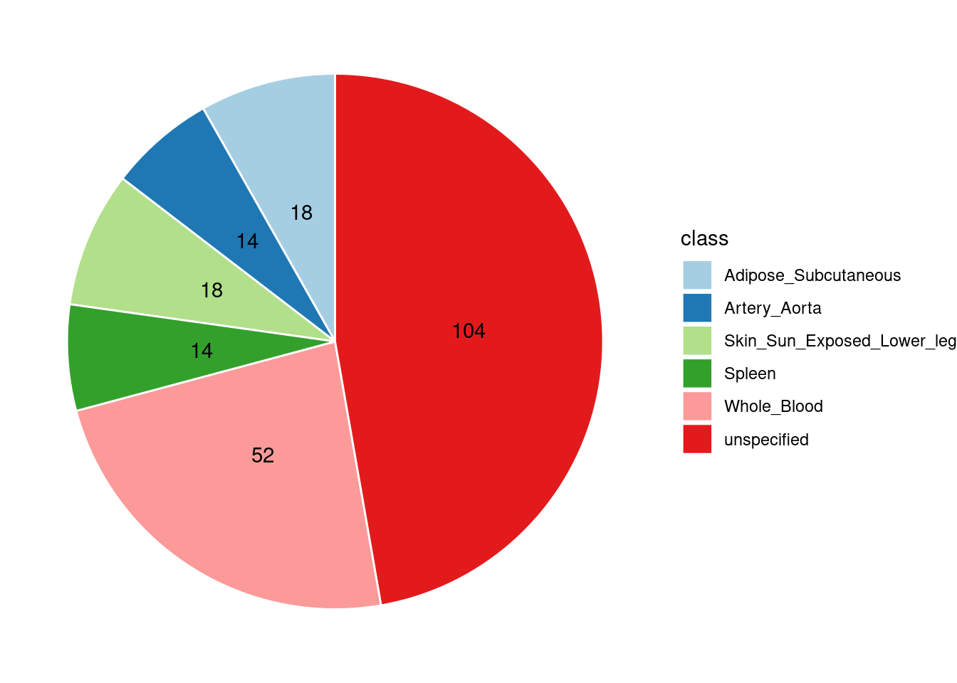
[1] "Whole_Blood"                "Adipose_Subcutaneous"
[3] "Artery_Aorta"               "Skin_Sun_Exposed_Lower_leg"
[5] "Spleen" 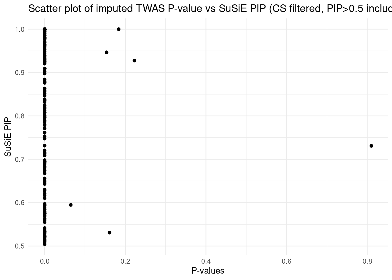
| Version | Author | Date |
|---|---|---|
| 9e83189 | XSun | 2024-06-13 |
Locus zoom plots for these 3 genes
https://uchicago.box.com/s/a1qej83jaabft9z7nqmzewzpsxrg6uui
https://uchicago.box.com/s/fzmv9ypzaa9vt7a4u0al37w7s77qrzdu
https://uchicago.box.com/s/70tk99ifpz7xshknh57u2pnf7jygx5zh
This PIP vs. p-value analysis suggests that some of the high PIP genes can be FPs. When the number of true signals in a region is < L (3 in our case), SuSiE will still try to report L results. This type of FP findings can be removed in the regular SuSiE by the CS filter. But it’s likely less effective in the cTWAS case, because our prior heavily favors genes. We may end up with a single gene in a CS with PIP > 0.95, then that gene will not be filtered by the purity filter.
One simple way to get the true number of signals is: run regular SuSiE (uniform prior) in a region, and obtain the number of CS from the results. This should be a pretty good estimate of the number of true signals.
By doing these, for these 3 regions,
For ING5, we have
estimated_L <- readRDS("/project/xinhe/xsun/multi_group_ctwas/5.multi_group_testing/results_preL/WBC-ieu-b-30/WBC-ieu-b-30.estimated_L.RDS")

sprintf("the pre-estimated L is %s", estimated_L["2:241210506-242147200"])
[1] "the pre-estimated L is 1"load("/project/xinhe/xsun/multi_group_ctwas/5.multi_group_testing/analy_results/ING5.preL.rdata")
DT::datatable(finemap_res_region_multi,caption = htmltools::tags$caption( style = 'caption-side: topleft; text-align = left; color:black;','Updated PIP (run with pre-estimated L)'),options = list(pageLength = 5) )For CCZ1, region 7:5814895-6534226 didn’t pass the screen_regions step
For ELMO1, region 7:36173929-37515581 didn’t pass the screen_regions step
Comparing with single group eQTL results
[1] "the top tissues from single group analyses are Whole_Blood,Adipose_Subcutaneous,Artery_Aorta,Skin_Sun_Exposed_Lower_leg,Spleen"
sessionInfo()R version 4.2.0 (2022-04-22)
Platform: x86_64-pc-linux-gnu (64-bit)
Running under: CentOS Linux 7 (Core)
Matrix products: default
BLAS/LAPACK: /software/openblas-0.3.13-el7-x86_64/lib/libopenblas_haswellp-r0.3.13.so
locale:
[1] C
attached base packages:
[1] stats graphics grDevices utils datasets methods base
other attached packages:
[1] gridExtra_2.3 RColorBrewer_1.1-3 forcats_0.5.1 stringr_1.5.1
[5] dplyr_1.1.4 purrr_1.0.2 readr_2.1.2 tidyr_1.3.0
[9] tibble_3.2.1 ggplot2_3.5.1 tidyverse_1.3.1 data.table_1.14.2
[13] ctwas_0.2.30
loaded via a namespace (and not attached):
[1] readxl_1.4.0 backports_1.4.1
[3] workflowr_1.7.0 BiocFileCache_2.4.0
[5] plyr_1.8.7 lazyeval_0.2.2
[7] crosstalk_1.2.0 BiocParallel_1.30.3
[9] GenomeInfoDb_1.39.9 LDlinkR_1.2.3
[11] digest_0.6.29 foreach_1.5.2
[13] ensembldb_2.20.2 htmltools_0.5.2
[15] fansi_1.0.3 magrittr_2.0.3
[17] memoise_2.0.1 doParallel_1.0.17
[19] tzdb_0.4.0 Biostrings_2.64.0
[21] modelr_0.1.8 matrixStats_0.62.0
[23] locuszoomr_0.2.1 prettyunits_1.1.1
[25] colorspace_2.0-3 blob_1.2.3
[27] rvest_1.0.2 rappdirs_0.3.3
[29] ggrepel_0.9.1 haven_2.5.0
[31] xfun_0.41 crayon_1.5.1
[33] RCurl_1.98-1.7 jsonlite_1.8.0
[35] zoo_1.8-10 iterators_1.0.14
[37] glue_1.6.2 gtable_0.3.0
[39] zlibbioc_1.42.0 XVector_0.36.0
[41] DelayedArray_0.22.0 BiocGenerics_0.42.0
[43] scales_1.3.0 DBI_1.2.2
[45] Rcpp_1.0.12 viridisLite_0.4.0
[47] progress_1.2.2 bit_4.0.4
[49] DT_0.22 stats4_4.2.0
[51] htmlwidgets_1.5.4 httr_1.4.3
[53] ellipsis_0.3.2 pkgconfig_2.0.3
[55] XML_3.99-0.14 farver_2.1.0
[57] sass_0.4.1 dbplyr_2.1.1
[59] utf8_1.2.2 tidyselect_1.2.0
[61] labeling_0.4.2 rlang_1.1.2
[63] later_1.3.0 AnnotationDbi_1.58.0
[65] munsell_0.5.0 pgenlibr_0.3.3
[67] cellranger_1.1.0 tools_4.2.0
[69] cachem_1.0.6 cli_3.6.1
[71] generics_0.1.2 RSQLite_2.3.1
[73] broom_0.8.0 evaluate_0.15
[75] fastmap_1.1.0 yaml_2.3.5
[77] knitr_1.39 bit64_4.0.5
[79] fs_1.5.2 KEGGREST_1.36.3
[81] AnnotationFilter_1.20.0 whisker_0.4
[83] xml2_1.3.3 biomaRt_2.54.1
[85] compiler_4.2.0 rstudioapi_0.13
[87] plotly_4.10.0 filelock_1.0.2
[89] curl_4.3.2 png_0.1-7
[91] reprex_2.0.1 bslib_0.3.1
[93] stringi_1.7.6 highr_0.9
[95] GenomicFeatures_1.48.3 lattice_0.20-45
[97] ProtGenerics_1.28.0 Matrix_1.5-3
[99] vctrs_0.6.5 pillar_1.9.0
[101] lifecycle_1.0.4 jquerylib_0.1.4
[103] cowplot_1.1.1 bitops_1.0-7
[105] irlba_2.3.5 httpuv_1.6.5
[107] rtracklayer_1.56.0 GenomicRanges_1.48.0
[109] R6_2.5.1 BiocIO_1.6.0
[111] promises_1.2.0.1 IRanges_2.30.0
[113] codetools_0.2-18 assertthat_0.2.1
[115] SummarizedExperiment_1.26.1 rprojroot_2.0.3
[117] rjson_0.2.21 withr_2.5.0
[119] GenomicAlignments_1.32.0 Rsamtools_2.12.0
[121] S4Vectors_0.34.0 GenomeInfoDbData_1.2.8
[123] parallel_4.2.0 hms_1.1.1
[125] grid_4.2.0 gggrid_0.2-0
[127] rmarkdown_2.25 MatrixGenerics_1.8.0
[129] logging_0.10-108 git2r_0.30.1
[131] mixsqp_0.3-43 Biobase_2.56.0
[133] lubridate_1.8.0 restfulr_0.0.14