Last updated: 2024-05-27

Checks: 6 1

Knit directory: multigroup_ctwas_analysis/

This reproducible R Markdown analysis was created with workflowr (version 1.7.0). The Checks tab describes the reproducibility checks that were applied when the results were created. The Past versions tab lists the development history.

R Markdown file: uncommitted changes

The R Markdown file has unstaged changes. To know which version of the R Markdown file created these results, you’ll want to first commit it to the Git repo. If you’re still working on the analysis, you can ignore this warning. When you’re finished, you can run wflow_publish to commit the R Markdown file and build the HTML.

Environment: empty

Great job! The global environment was empty. Objects defined in the global environment can affect the analysis in your R Markdown file in unknown ways. For reproduciblity it’s best to always run the code in an empty environment.

Seed: set.seed(20231112)

The command set.seed(20231112) was run prior to running the code in the R Markdown file. Setting a seed ensures that any results that rely on randomness, e.g. subsampling or permutations, are reproducible.

Session information: recorded

Great job! Recording the operating system, R version, and package versions is critical for reproducibility.

Cache: none

Nice! There were no cached chunks for this analysis, so you can be confident that you successfully produced the results during this run.

File paths: relative

Great job! Using relative paths to the files within your workflowr project makes it easier to run your code on other machines.

Repository version: 2986d3e

Great! You are using Git for version control. Tracking code development and connecting the code version to the results is critical for reproducibility.

The results in this page were generated with repository version 2986d3e. See the Past versions tab to see a history of the changes made to the R Markdown and HTML files.

Note that you need to be careful to ensure that all relevant files for the analysis have been committed to Git prior to generating the results (you can use wflow_publish or wflow_git_commit). workflowr only checks the R Markdown file, but you know if there are other scripts or data files that it depends on. Below is the status of the Git repository when the results were generated:


Ignored files:
    Ignored:    .Rhistory
    Ignored:    results/

Unstaged changes:
    Modified:   analysis/matching_tissue_v2.Rmd

Note that any generated files, e.g. HTML, png, CSS, etc., are not included in this status report because it is ok for generated content to have uncommitted changes.

These are the previous versions of the repository in which changes were made to the R Markdown (analysis/matching_tissue_v2.Rmd) and HTML (docs/matching_tissue_v2.html) files. If you’ve configured a remote Git repository (see ?wflow_git_remote), click on the hyperlinks in the table below to view the files as they were in that past version.

File	Version	Author	Date	Message
Rmd	2986d3e	XSun	2024-05-27	update
html	2986d3e	XSun	2024-05-27	update
Rmd	0c0d0e4	XSun	2024-05-27	update
html	0c0d0e4	XSun	2024-05-27	update
Rmd	e88634b	XSun	2024-05-17	update
html	e88634b	XSun	2024-05-17	update
Rmd	eb48b22	XSun	2024-05-17	update
html	eb48b22	XSun	2024-05-17	update
Rmd	4363587	XSun	2024-05-16	update
html	4363587	XSun	2024-05-16	update

Analysis settings

parameters

thin = 0.1
niter_prefit = 3
niter = 30
L = 5
group_prior_var_structure = “independent”
maxSNP = 20000
min_nonSNP_PIP = 0.5
protein-coding genes selected

Traits

aFib, IBD, LDL, SBP, SCZ, WBC

details

Weights

PredictDB, 32 tissues with sample size (RNASeq.and.Genotyped.samples below) >= 200

load("/project/xinhe/xsun/multi_group_ctwas/1.single_tissue/summary/para_pip08.rdata")
sum_all <- para_sum
colnames(sum_all)[ncol(sum_all)] <-"PVE(%)"
sum_all$`PVE(%)` <- as.numeric(sum_all$`PVE(%)`)*100

weights <- read.csv("/project/xinhe/xsun/ctwas/1.matching_tissue/results_data/gtex_samplesize.csv")
DT::datatable(weights,options = list(pageLength = 5))

num_top <- 10

Tissue-tissue correlation data

From MASH paper, PMID30478440

The MASH paper provides a matrix indicating the shared magnitude of eQTLs among tissues by computing the proportion of effects significant in either tissue that are within 2-fold magnitude of one another.

data download link (MASH matrix)

load("/project/xinhe/xsun/ctwas/1.matching_tissue/data/tissue_cor.rdata")
clrs <- colorRampPalette(rev(c("#D73027","#FC8D59","#FEE090","#FFFFBF",
                               "#E0F3F8","#91BFDB","#4575B4")))(64)

We filtered the correlation using 0.8 as cutoff.

Functions used

library(lattice)
library(gridExtra)
library(ggplot2)
get_correlation <- function(tissue1, tissue2, cor_matrix) {
  # Check if tissues are in the matrix and find their positions
  pos1 <- match(tissue1, colnames(cor_matrix))
  pos2 <- match(tissue2, rownames(cor_matrix))
  
  return(cor_matrix[pos2, pos1]) 
}

r2cutoff <- 0.8
filter_tissues <- function(tissue_list, cor_matrix) {
  filtered_list <- c(tissue_list[1]) # Start with the first tissue
  
  for (i in 2:length(tissue_list)) {
    high_correlation_found <- FALSE
    for (j in 1:length(filtered_list)) {
      if (!is.na(get_correlation(filtered_list[j], tissue_list[i], cor_matrix)) &&
          get_correlation(filtered_list[j], tissue_list[i], cor_matrix) > r2cutoff) {
        high_correlation_found <- TRUE
        break # Break the inner loop as high correlation is found
      }
    }
    
    if (!high_correlation_found) {
      filtered_list <- c(filtered_list, tissue_list[i])
    }
  }
  return(filtered_list)
}

fill_upper_triangle <- function(cor_matrix) {
    for (i in 1:nrow(cor_matrix)) {
        for (j in 1:ncol(cor_matrix)) {
            # Check if the upper triangle element is NA and the lower triangle element is not NA
            if (is.na(cor_matrix[i, j]) && !is.na(cor_matrix[j, i])) {
                # Copy the value from the lower triangle to the upper triangle
                cor_matrix[i, j] <- cor_matrix[j, i]
            }
        }
    }
    cor_matrix[lower.tri(cor_matrix)] <- NA
    return(cor_matrix)
}

combine_vectors <- function(vec1, vec_cor1, vec2, vec_cor2, pad_with_na = TRUE) {
  # Check if padding with NAs is required
  if (pad_with_na) {
    # Pad the shorter primary vector and its corresponding vector with NAs
    if (length(vec1) < length(vec2)) {
      extra_length <- length(vec2) - length(vec1)
      vec1 <- c(vec1, rep(NA, extra_length))
      vec_cor1 <- c(vec_cor1, rep(NA, extra_length))
    } else {
      extra_length <- length(vec1) - length(vec2)
      vec2 <- c(vec2, rep(NA, extra_length))
      vec_cor2 <- c(vec_cor2, rep(NA, extra_length))
    }
    # Combine the vectors into a matrix/data frame
    return(cbind(vec1, vec_cor1, vec2, vec_cor2))
  } else {
    # Combine the vectors into a list
    return(list(vec1=vec1, vec_cor1=vec_cor1, vec2=vec2, vec_cor2=vec_cor2))
  }
}

aFib

sum_cat <- sum_all[sum_all$trait =="aFib-ebi-a-GCST006414",]

DT::datatable(sum_cat,caption = htmltools::tags$caption( style = 'caption-side: topleft; text-align = left; color:black;  font-size:150% ;','summary for ctwas parameters and high pip genes (all tissues analyzed)'),options = list(pageLength = 5) )

Filtering based on the number of high PIP genes

sum_cat <- sum_cat[order(as.numeric(sum_cat$`#pip>0.8&incs`),decreasing = T),]

tissue_select <- sum_cat$tissue[num_top:1]
tissue_select <- tissue_select[tissue_select%in%rownames(lat)]

##heatmap
cor <- lat[tissue_select,tissue_select]
cor <- fill_upper_triangle(cor)
print(levelplot(cor,col.regions = clrs,xlab = "",ylab = "",
                colorkey = TRUE,main = "heatmap showing the tissue-tissue correlation"))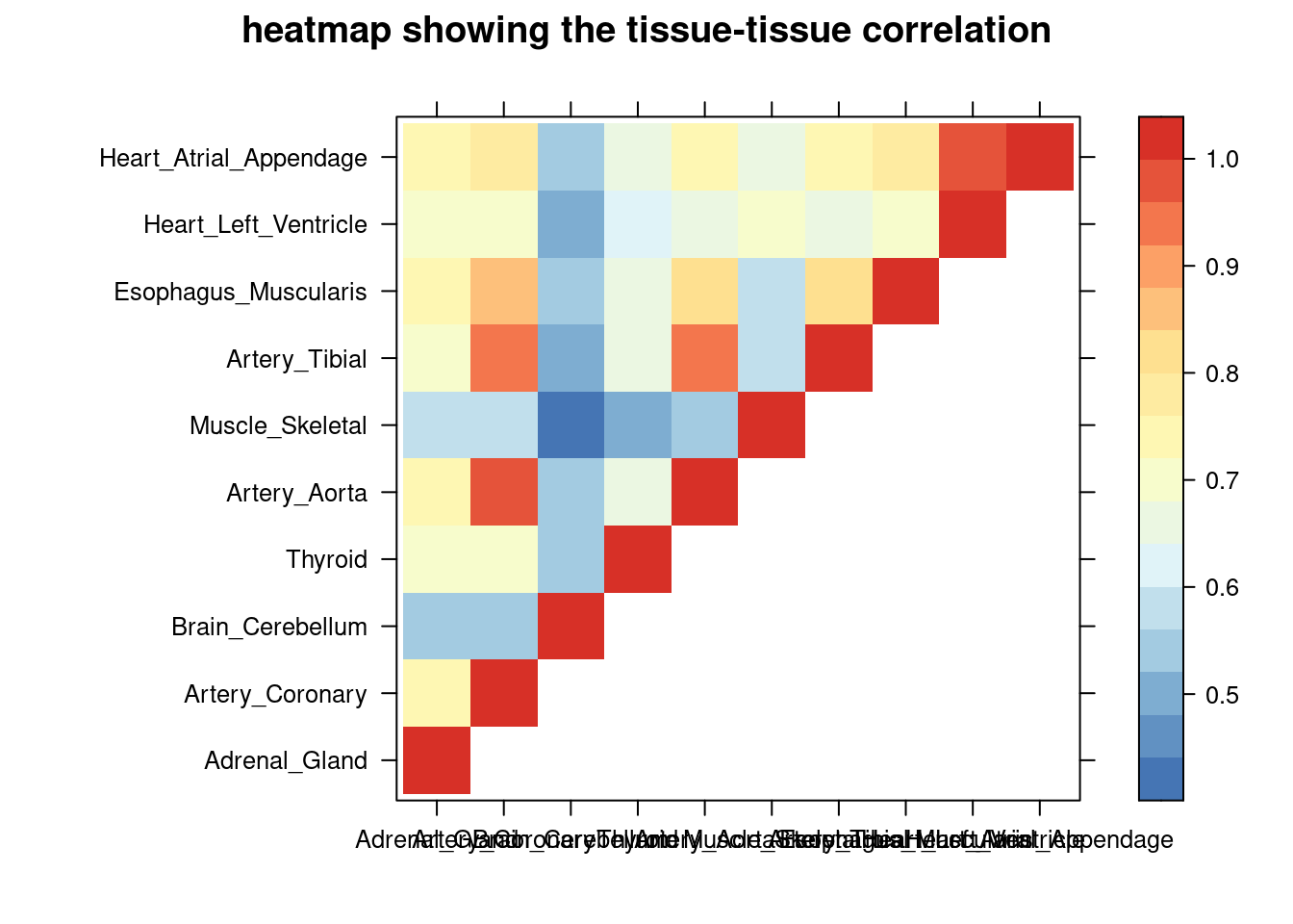

Version	Author	Date
4363587	XSun	2024-05-16

##cor matrix
cor <- cor[rev(tissue_select),rev(tissue_select)]
DT::datatable(cor,caption = htmltools::tags$caption( style = 'caption-side: topleft; text-align = left; color:black;  font-size:150% ;','tissue-tissue correlation matrix '),options = list(pageLength = 10) )

tissue_select_f1 <- sum_cat$tissue[1:num_top]
filtered_tissues <- filter_tissues(tissue_select_f1, cor)

tissue_select_f1_cor <- sum_cat$`#pip>0.8&incs`[sum_cat$tissue %in% tissue_select_f1 ]
filtered_tissues_cor <- sum_cat$`#pip>0.8&incs`[sum_cat$tissue %in% filtered_tissues ]
comb <- combine_vectors(tissue_select_f1, tissue_select_f1_cor, filtered_tissues, filtered_tissues_cor, pad_with_na = TRUE)
colnames(comb) <- c("without_filtering","#highpip_gene","filtered","#highpip_gene")


DT::datatable(comb,caption = htmltools::tags$caption( style = 'caption-side: left; text-align: left; color:black;  font-size:150% ;','Comparing the top tissue lists (with/without filtering by tissue correlation) '),options = list(pageLength = 10) )

Filtering based on PVE explained by genes

sum_cat <- sum_cat[order(as.numeric(sum_cat$group_pve),decreasing = T),]

tissue_select <- sum_cat$tissue[num_top:1]
tissue_select <- tissue_select[tissue_select%in%rownames(lat)]

##heatmap
cor <- lat[tissue_select,tissue_select]
cor <- fill_upper_triangle(cor)
print(levelplot(cor,col.regions = clrs,xlab = "",ylab = "",
                colorkey = TRUE,main = "heatmap showing the tissue-tissue correlation"))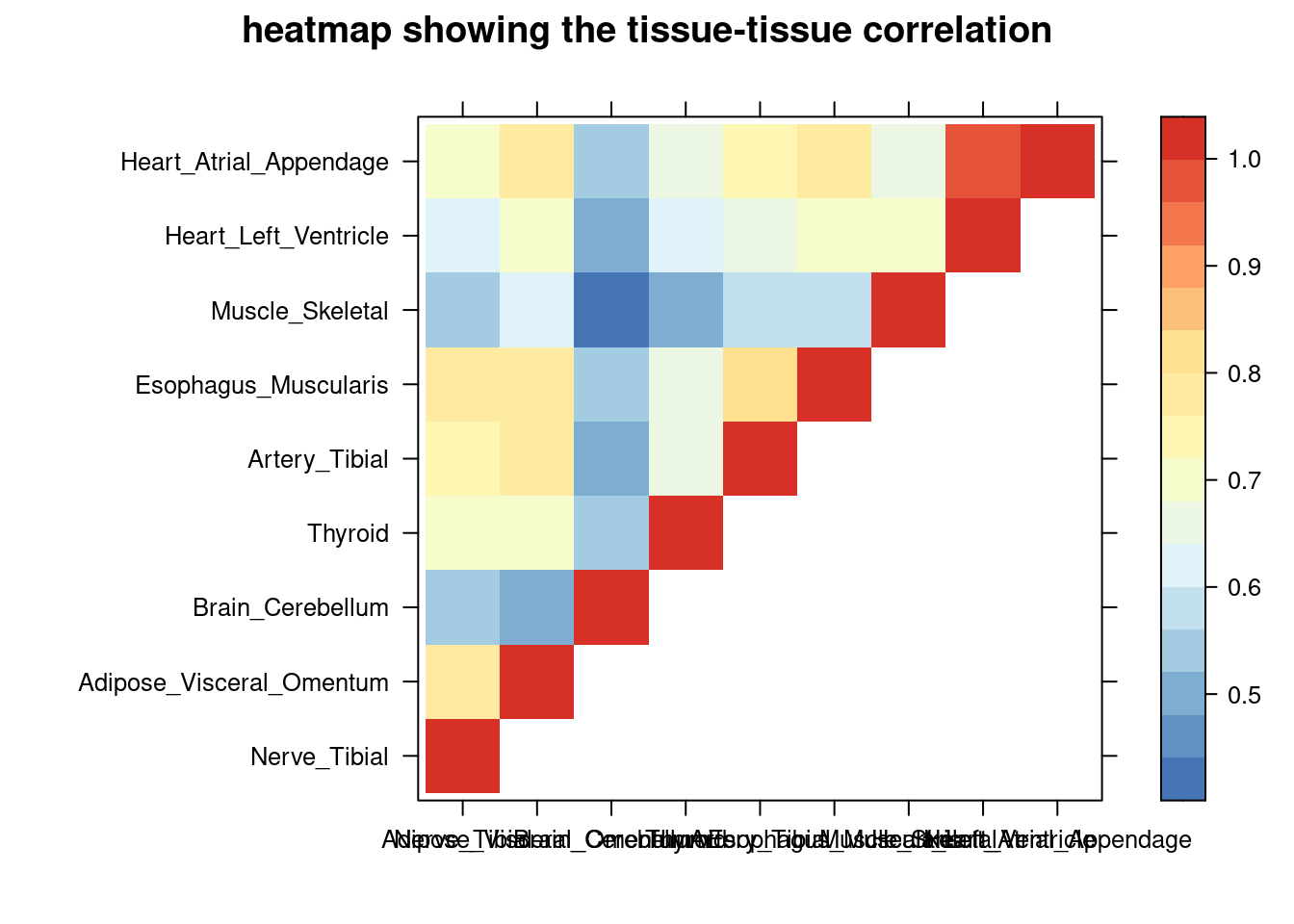

Version	Author	Date
4363587	XSun	2024-05-16

##cor matrix
cor <- cor[rev(tissue_select),rev(tissue_select)]
DT::datatable(cor,caption = htmltools::tags$caption( style = 'caption-side: topleft; text-align = left; color:black;  font-size:150% ;','tissue-tissue correlation matrix '),options = list(pageLength = 10) )

tissue_select_f1 <- sum_cat$tissue[1:num_top]
filtered_tissues <- filter_tissues(tissue_select_f1, cor)

tissue_select_f1_cor <- sum_cat$group_pve[sum_cat$tissue %in% tissue_select_f1 ]
filtered_tissues_cor <- sum_cat$group_pve[sum_cat$tissue %in% filtered_tissues ]
comb <- combine_vectors(tissue_select_f1, tissue_select_f1_cor, filtered_tissues, filtered_tissues_cor, pad_with_na = TRUE)
colnames(comb) <- c("without_filtering","PVE_gene","filtered","PVE_gene")


DT::datatable(comb,caption = htmltools::tags$caption( style = 'caption-side: left; text-align: left; color:black;  font-size:150% ;','Comparing the top tissue lists (with/without filtering by tissue correlation) '),options = list(pageLength = 10) )

IBD

sum_cat <- sum_all[sum_all$trait =="IBD-ebi-a-GCST004131",]

DT::datatable(sum_cat,caption = htmltools::tags$caption( style = 'caption-side: topleft; text-align = left; color:black;  font-size:150% ;','summary for ctwas parameters and high pip genes (all tissues analyzed)'),options = list(pageLength = 5) )

Filtering based on the number of high PIP genes

sum_cat <- sum_cat[order(as.numeric(sum_cat$`#pip>0.8&incs`),decreasing = T),]

tissue_select <- sum_cat$tissue[num_top:1]
tissue_select <- tissue_select[tissue_select%in%rownames(lat)]

##heatmap
cor <- lat[tissue_select,tissue_select]
cor <- fill_upper_triangle(cor)
print(levelplot(cor,col.regions = clrs,xlab = "",ylab = "",
                colorkey = TRUE,main = "heatmap showing the tissue-tissue correlation"))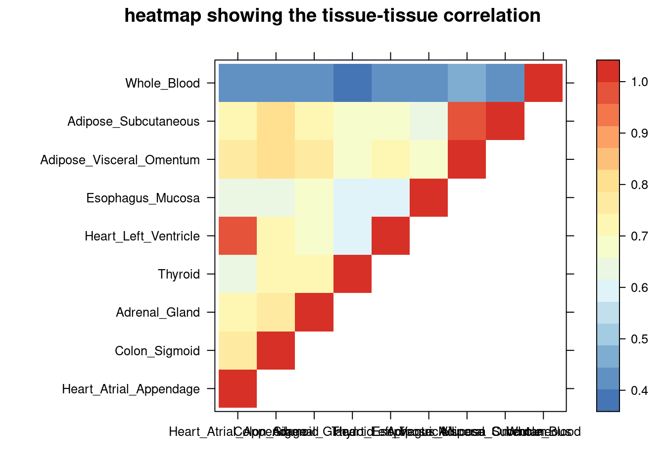

Version	Author	Date
4363587	XSun	2024-05-16

##cor matrix
cor <- cor[rev(tissue_select),rev(tissue_select)]
DT::datatable(cor,caption = htmltools::tags$caption( style = 'caption-side: topleft; text-align = left; color:black;  font-size:150% ;','tissue-tissue correlation matrix '),options = list(pageLength = 10) )

tissue_select_f1 <- sum_cat$tissue[1:num_top]
filtered_tissues <- filter_tissues(tissue_select_f1, cor)

tissue_select_f1_cor <- sum_cat$`#pip>0.8&incs`[sum_cat$tissue %in% tissue_select_f1 ]
filtered_tissues_cor <- sum_cat$`#pip>0.8&incs`[sum_cat$tissue %in% filtered_tissues ]
comb <- combine_vectors(tissue_select_f1, tissue_select_f1_cor, filtered_tissues, filtered_tissues_cor, pad_with_na = TRUE)
colnames(comb) <- c("without_filtering","#highpip_gene","filtered","#highpip_gene")


DT::datatable(comb,caption = htmltools::tags$caption( style = 'caption-side: left; text-align: left; color:black;  font-size:150% ;','Comparing the top tissue lists (with/without filtering by tissue correlation) '),options = list(pageLength = 10) )

Filtering based on PVE explained by genes

sum_cat <- sum_cat[order(as.numeric(sum_cat$group_pve),decreasing = T),]

tissue_select <- sum_cat$tissue[num_top:1]
tissue_select <- tissue_select[tissue_select%in%rownames(lat)]

##heatmap
cor <- lat[tissue_select,tissue_select]
cor <- fill_upper_triangle(cor)
print(levelplot(cor,col.regions = clrs,xlab = "",ylab = "",
                colorkey = TRUE,main = "heatmap showing the tissue-tissue correlation"))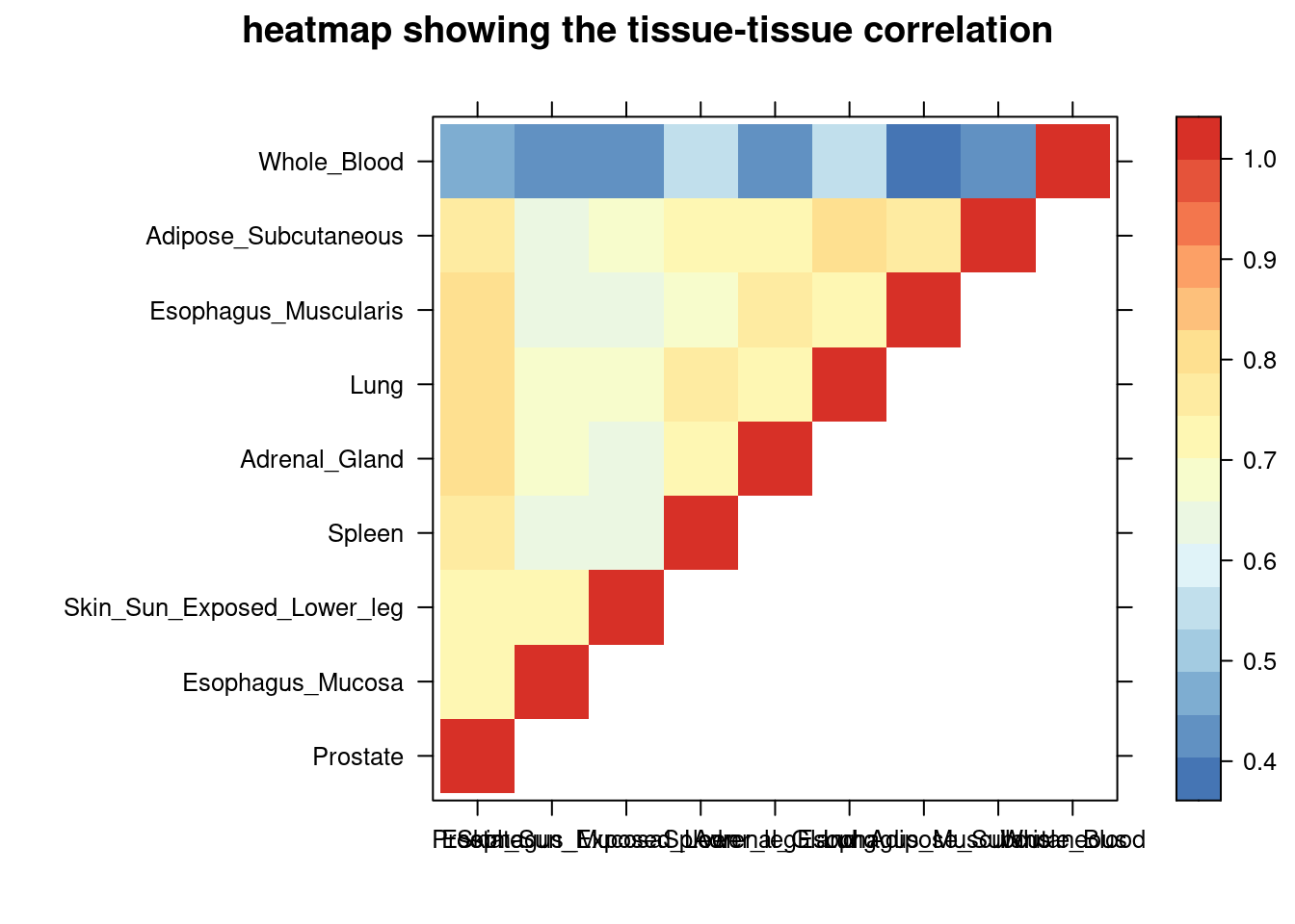

Version	Author	Date
4363587	XSun	2024-05-16

##cor matrix
cor <- cor[rev(tissue_select),rev(tissue_select)]
DT::datatable(cor,caption = htmltools::tags$caption( style = 'caption-side: topleft; text-align = left; color:black;  font-size:150% ;','tissue-tissue correlation matrix '),options = list(pageLength = 10) )

tissue_select_f1 <- sum_cat$tissue[1:num_top]
filtered_tissues <- filter_tissues(tissue_select_f1, cor)

tissue_select_f1_cor <- sum_cat$group_pve[sum_cat$tissue %in% tissue_select_f1 ]
filtered_tissues_cor <- sum_cat$group_pve[sum_cat$tissue %in% filtered_tissues ]
comb <- combine_vectors(tissue_select_f1, tissue_select_f1_cor, filtered_tissues, filtered_tissues_cor, pad_with_na = TRUE)
colnames(comb) <- c("without_filtering","PVE_gene","filtered","PVE_gene")


DT::datatable(comb,caption = htmltools::tags$caption( style = 'caption-side: left; text-align: left; color:black;  font-size:150% ;','Comparing the top tissue lists (with/without filtering by tissue correlation) '),options = list(pageLength = 10) )

LDL

sum_cat <- sum_all[sum_all$trait =="LDL-ukb-d-30780_irnt",]

DT::datatable(sum_cat,caption = htmltools::tags$caption( style = 'caption-side: topleft; text-align = left; color:black;  font-size:150% ;','summary for ctwas parameters and high pip genes (all tissues analyzed)'),options = list(pageLength = 5) )

Filtering based on the number of high PIP genes

sum_cat <- sum_cat[order(as.numeric(sum_cat$`#pip>0.8&incs`),decreasing = T),]

tissue_select <- sum_cat$tissue[num_top:1]
tissue_select <- tissue_select[tissue_select%in%rownames(lat)]

##heatmap
cor <- lat[tissue_select,tissue_select]
cor <- fill_upper_triangle(cor)
print(levelplot(cor,col.regions = clrs,xlab = "",ylab = "",
                colorkey = TRUE,main = "heatmap showing the tissue-tissue correlation"))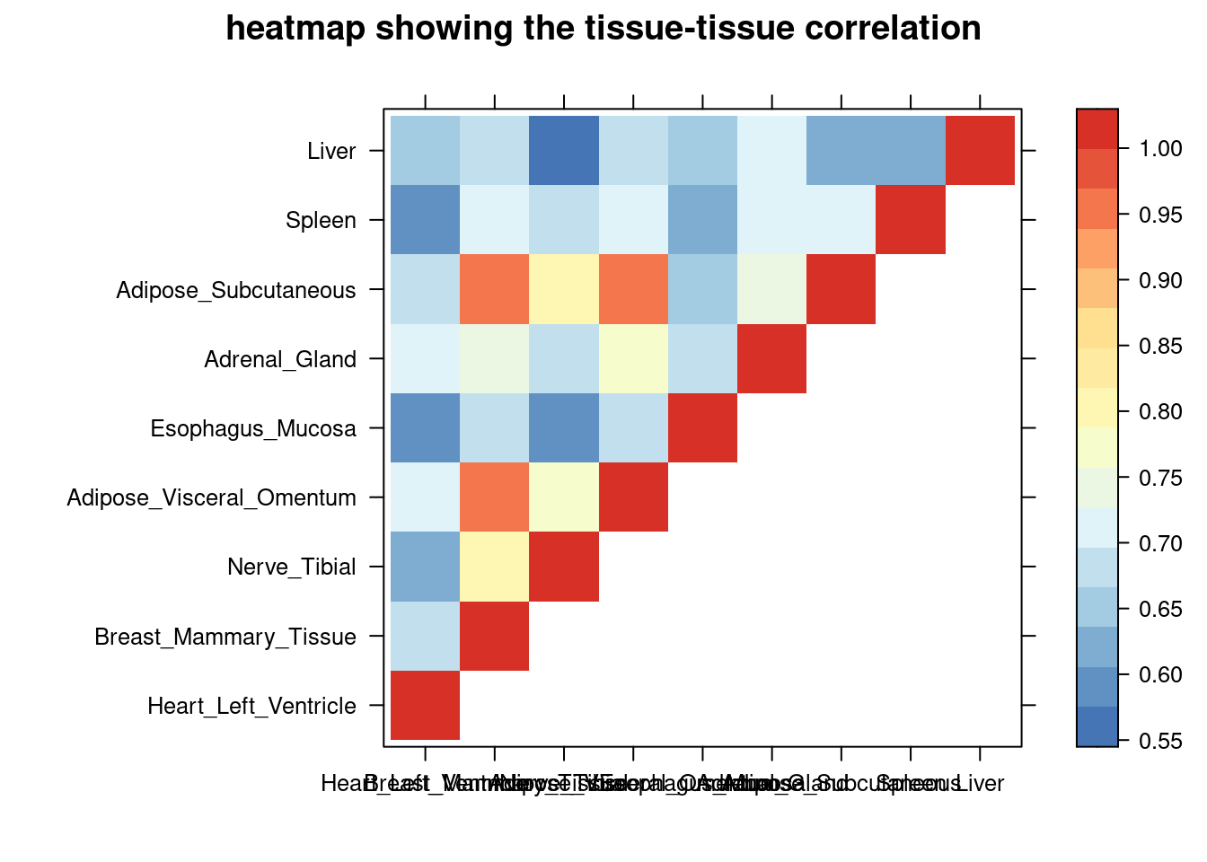

Version	Author	Date
4363587	XSun	2024-05-16

##cor matrix
cor <- cor[rev(tissue_select),rev(tissue_select)]
DT::datatable(cor,caption = htmltools::tags$caption( style = 'caption-side: topleft; text-align = left; color:black;  font-size:150% ;','tissue-tissue correlation matrix '),options = list(pageLength = 10) )

tissue_select_f1 <- sum_cat$tissue[1:num_top]
filtered_tissues <- filter_tissues(tissue_select_f1, cor)

tissue_select_f1_cor <- sum_cat$`#pip>0.8&incs`[sum_cat$tissue %in% tissue_select_f1 ]
filtered_tissues_cor <- sum_cat$`#pip>0.8&incs`[sum_cat$tissue %in% filtered_tissues ]
comb <- combine_vectors(tissue_select_f1, tissue_select_f1_cor, filtered_tissues, filtered_tissues_cor, pad_with_na = TRUE)
colnames(comb) <- c("without_filtering","#highpip_gene","filtered","#highpip_gene")


DT::datatable(comb,caption = htmltools::tags$caption( style = 'caption-side: left; text-align: left; color:black;  font-size:150% ;','Comparing the top tissue lists (with/without filtering by tissue correlation) '),options = list(pageLength = 10) )

Filtering based on PVE explained by genes

sum_cat <- sum_cat[order(as.numeric(sum_cat$group_pve),decreasing = T),]

tissue_select <- sum_cat$tissue[num_top:1]
tissue_select <- tissue_select[tissue_select%in%rownames(lat)]

##heatmap
cor <- lat[tissue_select,tissue_select]
cor <- fill_upper_triangle(cor)
print(levelplot(cor,col.regions = clrs,xlab = "",ylab = "",
                colorkey = TRUE,main = "heatmap showing the tissue-tissue correlation"))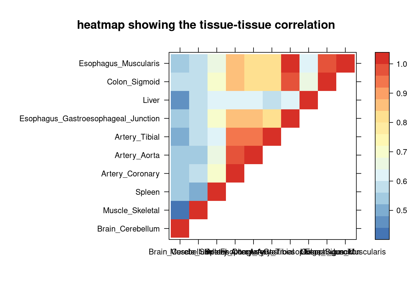

Version	Author	Date
4363587	XSun	2024-05-16

##cor matrix
cor <- cor[rev(tissue_select),rev(tissue_select)]
DT::datatable(cor,caption = htmltools::tags$caption( style = 'caption-side: topleft; text-align = left; color:black;  font-size:150% ;','tissue-tissue correlation matrix '),options = list(pageLength = 10) )

tissue_select_f1 <- sum_cat$tissue[1:num_top]
filtered_tissues <- filter_tissues(tissue_select_f1, cor)

tissue_select_f1_cor <- sum_cat$group_pve[sum_cat$tissue %in% tissue_select_f1 ]
filtered_tissues_cor <- sum_cat$group_pve[sum_cat$tissue %in% filtered_tissues ]
comb <- combine_vectors(tissue_select_f1, tissue_select_f1_cor, filtered_tissues, filtered_tissues_cor, pad_with_na = TRUE)
colnames(comb) <- c("without_filtering","PVE_gene","filtered","PVE_gene")


DT::datatable(comb,caption = htmltools::tags$caption( style = 'caption-side: left; text-align: left; color:black;  font-size:150% ;','Comparing the top tissue lists (with/without filtering by tissue correlation) '),options = list(pageLength = 10) )

SBP

sum_cat <- sum_all[sum_all$trait =="SBP-ukb-a-360",]

DT::datatable(sum_cat,caption = htmltools::tags$caption( style = 'caption-side: topleft; text-align = left; color:black;  font-size:150% ;','summary for ctwas parameters and high pip genes (all tissues analyzed)'),options = list(pageLength = 5) )

Filtering based on the number of high PIP genes

sum_cat <- sum_cat[order(as.numeric(sum_cat$`#pip>0.8&incs`),decreasing = T),]

tissue_select <- sum_cat$tissue[num_top:1]
tissue_select <- tissue_select[tissue_select%in%rownames(lat)]

##heatmap
cor <- lat[tissue_select,tissue_select]
cor <- fill_upper_triangle(cor)
print(levelplot(cor,col.regions = clrs,xlab = "",ylab = "",
                colorkey = TRUE,main = "heatmap showing the tissue-tissue correlation"))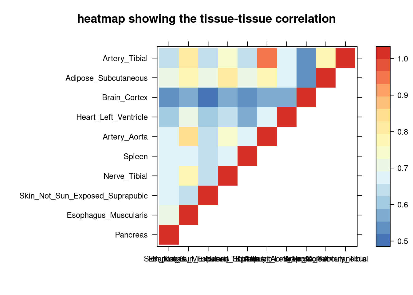

Version	Author	Date
4363587	XSun	2024-05-16

##cor matrix
cor <- cor[rev(tissue_select),rev(tissue_select)]
DT::datatable(cor,caption = htmltools::tags$caption( style = 'caption-side: topleft; text-align = left; color:black;  font-size:150% ;','tissue-tissue correlation matrix '),options = list(pageLength = 10) )

tissue_select_f1 <- sum_cat$tissue[1:num_top]
filtered_tissues <- filter_tissues(tissue_select_f1, cor)

tissue_select_f1_cor <- sum_cat$`#pip>0.8&incs`[sum_cat$tissue %in% tissue_select_f1 ]
filtered_tissues_cor <- sum_cat$`#pip>0.8&incs`[sum_cat$tissue %in% filtered_tissues ]
comb <- combine_vectors(tissue_select_f1, tissue_select_f1_cor, filtered_tissues, filtered_tissues_cor, pad_with_na = TRUE)
colnames(comb) <- c("without_filtering","#highpip_gene","filtered","#highpip_gene")


DT::datatable(comb,caption = htmltools::tags$caption( style = 'caption-side: left; text-align: left; color:black;  font-size:150% ;','Comparing the top tissue lists (with/without filtering by tissue correlation) '),options = list(pageLength = 10) )

Filtering based on PVE explained by genes

sum_cat <- sum_cat[order(as.numeric(sum_cat$group_pve),decreasing = T),]

tissue_select <- sum_cat$tissue[num_top:1]
tissue_select <- tissue_select[tissue_select%in%rownames(lat)]

##heatmap
cor <- lat[tissue_select,tissue_select]
cor <- fill_upper_triangle(cor)
print(levelplot(cor,col.regions = clrs,xlab = "",ylab = "",
                colorkey = TRUE,main = "heatmap showing the tissue-tissue correlation"))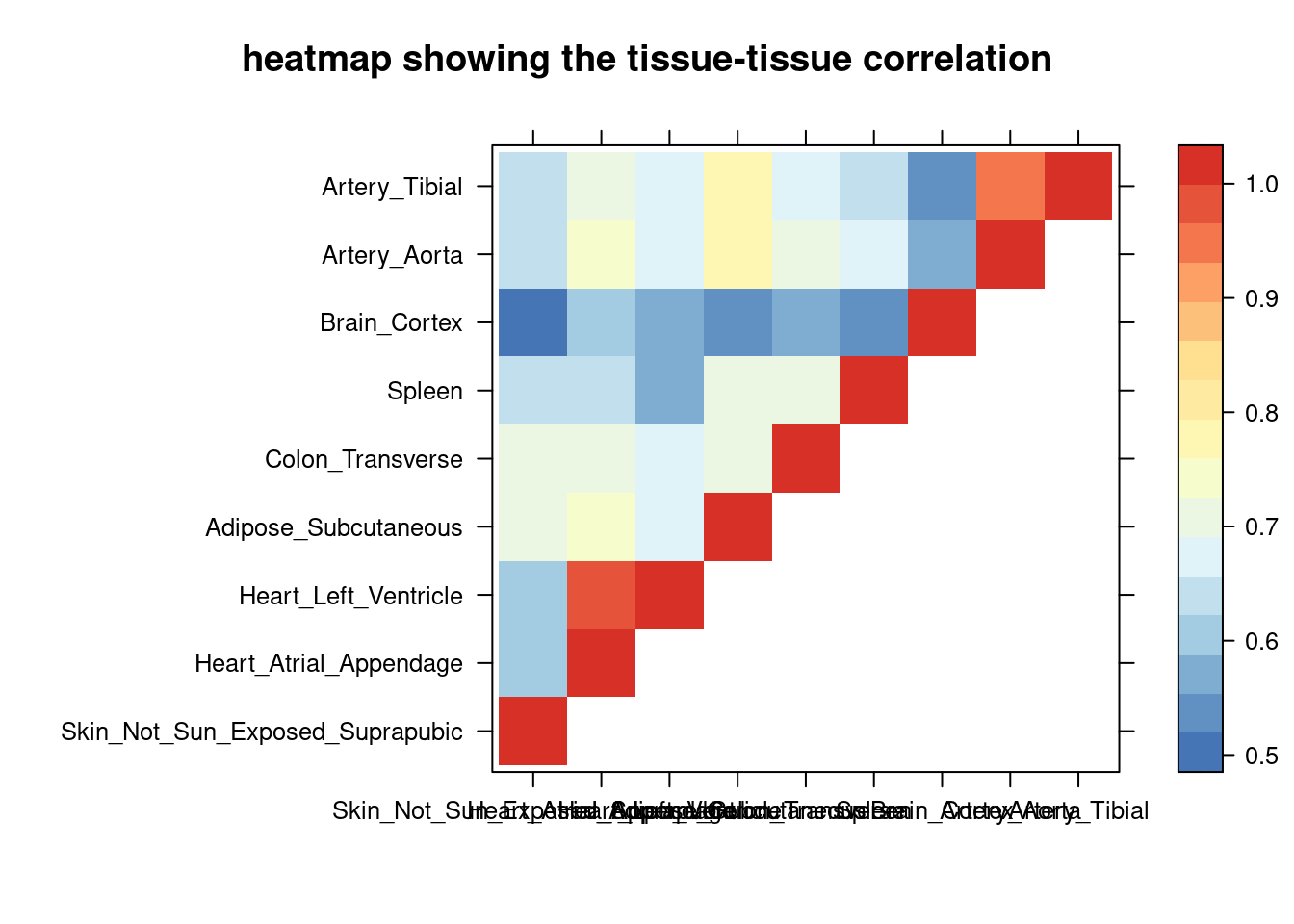

Version	Author	Date
4363587	XSun	2024-05-16

##cor matrix
cor <- cor[rev(tissue_select),rev(tissue_select)]
DT::datatable(cor,caption = htmltools::tags$caption( style = 'caption-side: topleft; text-align = left; color:black;  font-size:150% ;','tissue-tissue correlation matrix '),options = list(pageLength = 10) )

tissue_select_f1 <- sum_cat$tissue[1:num_top]
filtered_tissues <- filter_tissues(tissue_select_f1, cor)

tissue_select_f1_cor <- sum_cat$group_pve[sum_cat$tissue %in% tissue_select_f1 ]
filtered_tissues_cor <- sum_cat$group_pve[sum_cat$tissue %in% filtered_tissues ]
comb <- combine_vectors(tissue_select_f1, tissue_select_f1_cor, filtered_tissues, filtered_tissues_cor, pad_with_na = TRUE)
colnames(comb) <- c("without_filtering","PVE_gene","filtered","PVE_gene")


DT::datatable(comb,caption = htmltools::tags$caption( style = 'caption-side: left; text-align: left; color:black;  font-size:150% ;','Comparing the top tissue lists (with/without filtering by tissue correlation) '),options = list(pageLength = 10) )

SCZ

sum_cat <- sum_all[sum_all$trait =="SCZ-ieu-b-5102",]

DT::datatable(sum_cat,caption = htmltools::tags$caption( style = 'caption-side: topleft; text-align = left; color:black;  font-size:150% ;','summary for ctwas parameters and high pip genes (all tissues analyzed)'),options = list(pageLength = 5) )

Filtering based on the number of high PIP genes

sum_cat <- sum_cat[order(as.numeric(sum_cat$`#pip>0.8&incs`),decreasing = T),]

tissue_select <- sum_cat$tissue[num_top:1]
tissue_select <- tissue_select[tissue_select%in%rownames(lat)]

##heatmap
cor <- lat[tissue_select,tissue_select]
cor <- fill_upper_triangle(cor)
print(levelplot(cor,col.regions = clrs,xlab = "",ylab = "",
                colorkey = TRUE,main = "heatmap showing the tissue-tissue correlation"))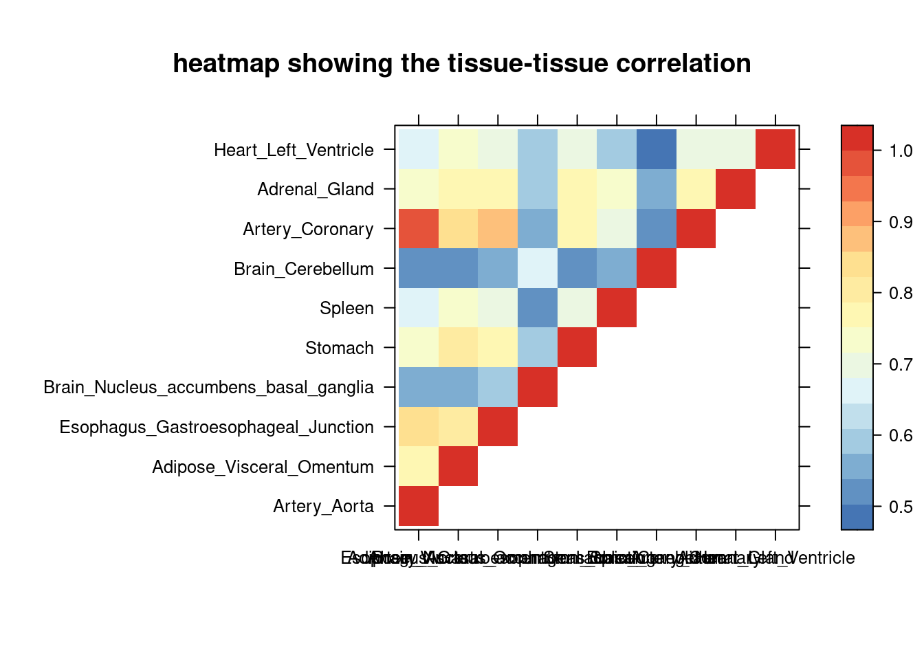

Version	Author	Date
4363587	XSun	2024-05-16

##cor matrix
cor <- cor[rev(tissue_select),rev(tissue_select)]
DT::datatable(cor,caption = htmltools::tags$caption( style = 'caption-side: topleft; text-align = left; color:black;  font-size:150% ;','tissue-tissue correlation matrix '),options = list(pageLength = 10) )

tissue_select_f1 <- sum_cat$tissue[1:num_top]
filtered_tissues <- filter_tissues(tissue_select_f1, cor)

tissue_select_f1_cor <- sum_cat$`#pip>0.8&incs`[sum_cat$tissue %in% tissue_select_f1 ]
filtered_tissues_cor <- sum_cat$`#pip>0.8&incs`[sum_cat$tissue %in% filtered_tissues ]
comb <- combine_vectors(tissue_select_f1, tissue_select_f1_cor, filtered_tissues, filtered_tissues_cor, pad_with_na = TRUE)
colnames(comb) <- c("without_filtering","#highpip_gene","filtered","#highpip_gene")


DT::datatable(comb,caption = htmltools::tags$caption( style = 'caption-side: left; text-align: left; color:black;  font-size:150% ;','Comparing the top tissue lists (with/without filtering by tissue correlation) '),options = list(pageLength = 10) )

Filtering based on PVE explained by genes

sum_cat <- sum_cat[order(as.numeric(sum_cat$group_pve),decreasing = T),]

tissue_select <- sum_cat$tissue[num_top:1]
tissue_select <- tissue_select[tissue_select%in%rownames(lat)]

##heatmap
cor <- lat[tissue_select,tissue_select]
cor <- fill_upper_triangle(cor)
print(levelplot(cor,col.regions = clrs,xlab = "",ylab = "",
                colorkey = TRUE,main = "heatmap showing the tissue-tissue correlation"))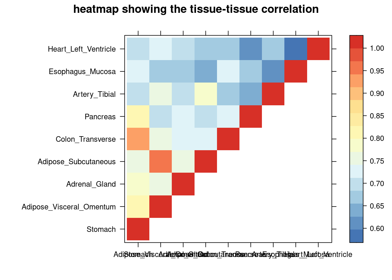

Version	Author	Date
4363587	XSun	2024-05-16

##cor matrix
cor <- cor[rev(tissue_select),rev(tissue_select)]
DT::datatable(cor,caption = htmltools::tags$caption( style = 'caption-side: topleft; text-align = left; color:black;  font-size:150% ;','tissue-tissue correlation matrix '),options = list(pageLength = 10) )

tissue_select_f1 <- sum_cat$tissue[1:num_top]
filtered_tissues <- filter_tissues(tissue_select_f1, cor)

tissue_select_f1_cor <- sum_cat$group_pve[sum_cat$tissue %in% tissue_select_f1 ]
filtered_tissues_cor <- sum_cat$group_pve[sum_cat$tissue %in% filtered_tissues ]
comb <- combine_vectors(tissue_select_f1, tissue_select_f1_cor, filtered_tissues, filtered_tissues_cor, pad_with_na = TRUE)
colnames(comb) <- c("without_filtering","PVE_gene","filtered","PVE_gene")


DT::datatable(comb,caption = htmltools::tags$caption( style = 'caption-side: left; text-align: left; color:black;  font-size:150% ;','Comparing the top tissue lists (with/without filtering by tissue correlation) '),options = list(pageLength = 10) )

WBC

sum_cat <- sum_all[sum_all$trait =="WBC-ieu-b-30",]

DT::datatable(sum_cat,caption = htmltools::tags$caption( style = 'caption-side: topleft; text-align = left; color:black;  font-size:150% ;','summary for ctwas parameters and high pip genes (all tissues analyzed)'),options = list(pageLength = 5) )

Filtering based on the number of high PIP genes

sum_cat <- sum_cat[order(as.numeric(sum_cat$`#pip>0.8&incs`),decreasing = T),]

tissue_select <- sum_cat$tissue[num_top:1]
tissue_select <- tissue_select[tissue_select%in%rownames(lat)]

##heatmap
cor <- lat[tissue_select,tissue_select]
cor <- fill_upper_triangle(cor)
print(levelplot(cor,col.regions = clrs,xlab = "",ylab = "",
                colorkey = TRUE,main = "heatmap showing the tissue-tissue correlation"))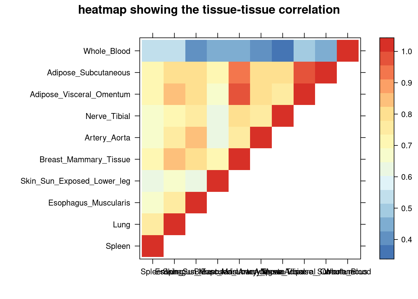

Version	Author	Date
4363587	XSun	2024-05-16

##cor matrix
cor <- cor[rev(tissue_select),rev(tissue_select)]
DT::datatable(cor,caption = htmltools::tags$caption( style = 'caption-side: topleft; text-align = left; color:black;  font-size:150% ;','tissue-tissue correlation matrix '),options = list(pageLength = 10) )

tissue_select_f1 <- sum_cat$tissue[1:num_top]
filtered_tissues <- filter_tissues(tissue_select_f1, cor)

tissue_select_f1_cor <- sum_cat$`#pip>0.8&incs`[sum_cat$tissue %in% tissue_select_f1 ]
filtered_tissues_cor <- sum_cat$`#pip>0.8&incs`[sum_cat$tissue %in% filtered_tissues ]
comb <- combine_vectors(tissue_select_f1, tissue_select_f1_cor, filtered_tissues, filtered_tissues_cor, pad_with_na = TRUE)
colnames(comb) <- c("without_filtering","#highpip_gene","filtered","#highpip_gene")


DT::datatable(comb,caption = htmltools::tags$caption( style = 'caption-side: left; text-align: left; color:black;  font-size:150% ;','Comparing the top tissue lists (with/without filtering by tissue correlation) '),options = list(pageLength = 10) )

Filtering based on PVE explained by genes

sum_cat <- sum_cat[order(as.numeric(sum_cat$group_pve),decreasing = T),]

tissue_select <- sum_cat$tissue[num_top:1]
tissue_select <- tissue_select[tissue_select%in%rownames(lat)]

##heatmap
cor <- lat[tissue_select,tissue_select]
cor <- fill_upper_triangle(cor)
print(levelplot(cor,col.regions = clrs,xlab = "",ylab = "",
                colorkey = TRUE,main = "heatmap showing the tissue-tissue correlation"))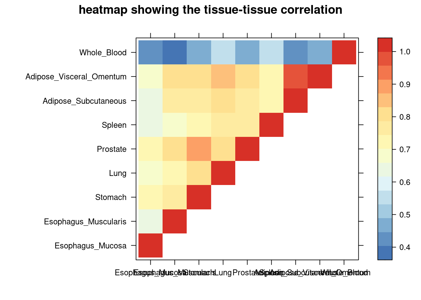

Version	Author	Date
4363587	XSun	2024-05-16

##cor matrix
cor <- cor[rev(tissue_select),rev(tissue_select)]
DT::datatable(cor,caption = htmltools::tags$caption( style = 'caption-side: topleft; text-align = left; color:black;  font-size:150% ;','tissue-tissue correlation matrix '),options = list(pageLength = 10) )

tissue_select_f1 <- sum_cat$tissue[1:num_top]
filtered_tissues <- filter_tissues(tissue_select_f1, cor)

tissue_select_f1_cor <- sum_cat$group_pve[sum_cat$tissue %in% tissue_select_f1 ]
filtered_tissues_cor <- sum_cat$group_pve[sum_cat$tissue %in% filtered_tissues ]
comb <- combine_vectors(tissue_select_f1, tissue_select_f1_cor, filtered_tissues, filtered_tissues_cor, pad_with_na = TRUE)
colnames(comb) <- c("without_filtering","PVE_gene","filtered","PVE_gene")


DT::datatable(comb,caption = htmltools::tags$caption( style = 'caption-side: left; text-align: left; color:black;  font-size:150% ;','Comparing the top tissue lists (with/without filtering by tissue correlation) '),options = list(pageLength = 10) )

Selected Tissues

Trait	Number of Tissues	Tissue	# of high pip genes (in cs)	PVE (if same in number of high pip genes)
aFib	5	Heart_Atrial_Appendage	23
		Esophagus_Muscularis	14
		Muscle_Skeletal	11
		Thyroid	12
		Brain_Cerebellum	10
IBD	6	Cells_Cultured_fibroblasts	16
		Whole_Blood	14
		Adipose_Subcutaneous	12
		Esophagus_Mucosa	8	0.025728
		Heart_Left_Ventricle	8	0.023978
		Thyroid	8	0.016433
LDL	5	Liver	40
		Spleen	24
		Adipose_Subcutaneous	21
		Adrenal_Gland	19
		Esophagus_Mucosa	19
SBP	5	Artery_Tibial	35
		Adipose_Subcutaneous	29
		Brain_Cortex	29
		Heart_Left_Ventricle	25
		Spleen	21
SCZ	6	Heart_Left_Ventricle	23
		Adrenal_Gland	22
		Artery_Coronary	16
		Brain_Cerebellum	16
		Spleen	15	0.01715
		Stomach	15	0.01868
WBC	5	Whole_Blood	109
		Adipose_Subcutaneous	68
		Artery_Aorta	56
		Skin_Sun_Exposed_Lower_leg	54
		Spleen	52

Comparing with the results from package V1

The different settings running these analyses:

Weights

When running V1: we used weights for nolnc genes (protein-coding and pseudogenes left)
When running V2: we just used weights for protein-coding genes, which are a bit fewer.

Region merge

When running V1: we merged regions having boundary genes.
When running V2: we didn’t do post processing.

load("/project/xinhe/xsun/ctwas/1.matching_tissue/results_data/summary_table.rd")
colnames(sum_all)[8] <- "num_gene_susiepip08"
results_v1 <- sum_all

load("/project/xinhe/xsun/ctwas/1.matching_tissue/results_data/summary_table_cs.rdata")
colnames(sum_all)[1:2] <- c("traits", "weights")
# Merge the data frames
results_v1 <- merge(results_v1, sum_all, by = c("traits", "weights"), all.x = TRUE)


load("/project/xinhe/xsun/multi_group_ctwas/1.single_tissue/summary/para_pip08.rdata")
results_v2 <- para_sum

results_v1 <- results_v1[results_v1$traits %in% results_v2$trait,]
results_v1 <- results_v1[results_v1$weights %in% results_v2$tissue,]


# Create a combined key column in both data frames
results_v1$key <- paste(results_v1$traits, results_v1$weights, sep = "_")
results_v2$key <- paste(results_v2$trait, results_v2$tissue, sep = "_")

# Sort each data frame by the combined key
results_v1_sorted <- results_v1[order(results_v1$key), ]
results_v2_sorted <- results_v2[order(results_v2$key), ]

# Optionally, drop the key column if it's no longer needed
results_v1_sorted$key <- NULL
results_v2_sorted$key <- NULL

results_v1_sorted$group_pve_gene <- as.numeric(results_v1_sorted$group_pve_gene)
results_v2_sorted$group_pve <- as.numeric(results_v2_sorted$group_pve)
p1 <- ggplot(data = NULL, aes(x = results_v1_sorted$group_pve_gene, y = results_v2_sorted$group_pve)) +
  geom_point() +
  geom_abline(slope = 1, intercept = 0, color = "red") +
  labs(x = "group_pve (V1)", y = "group_pve (V2)") +
  theme_minimal()

results_v1_sorted$num_gene_susiepip08 <- as.numeric(results_v1_sorted$num_gene_susiepip08)
results_v2_sorted$`#pip>0.8` <- as.numeric(results_v2_sorted$`#pip>0.8`)
# Plot 2: num_gene_susiepip08 vs. #pip>0.8
p2 <- ggplot(data = NULL, aes(x = results_v1_sorted$num_gene_susiepip08, y = results_v2_sorted$`#pip>0.8`)) +
  geom_point() +
  geom_abline(slope = 1, intercept = 0, color = "red") +
  labs(x = "#pip>0.8 (V1)", y = "#pip>0.8 (V2)") +
  theme_minimal()

results_v1_sorted$num_gene_08_cs <- as.numeric(results_v1_sorted$num_gene_08_cs)
results_v2_sorted$`#pip>0.8&incs` <- as.numeric(results_v2_sorted$`#pip>0.8&incs`)
# Plot 3: num_gene_08_cs vs. #pip>0.8&incs
p3 <- ggplot(data = NULL, aes(x = results_v1_sorted$num_gene_08_cs, y = results_v2_sorted$`#pip>0.8&incs`)) +
  geom_point() +
  geom_abline(slope = 1, intercept = 0, color = "red") +
  labs(x = "#pip>0.8&incs (V1)", y = "#pip>0.8&incs (V2)") +
  theme_minimal()

grid.arrange(p1, p2, p3, ncol = 3)

Warning: Removed 1 row containing missing values or values outside the scale range
(`geom_point()`).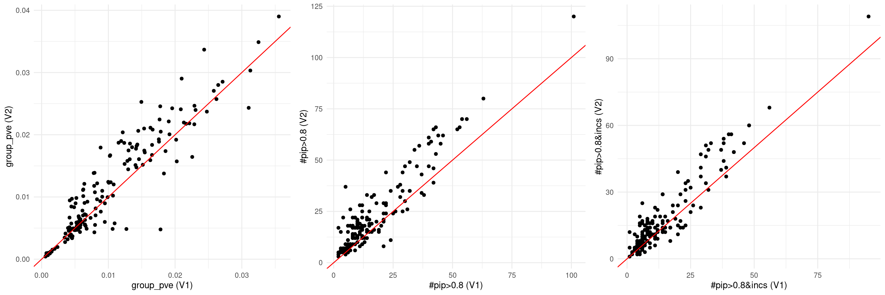

Version	Author	Date
e88634b	XSun	2024-05-17

sessionInfo()

R version 4.2.0 (2022-04-22)
Platform: x86_64-pc-linux-gnu (64-bit)
Running under: CentOS Linux 7 (Core)

Matrix products: default
BLAS/LAPACK: /software/openblas-0.3.13-el7-x86_64/lib/libopenblas_haswellp-r0.3.13.so

locale:
[1] C

attached base packages:
[1] stats     graphics  grDevices utils     datasets  methods   base     

other attached packages:
[1] ggplot2_3.5.1   gridExtra_2.3   lattice_0.20-45

loaded via a namespace (and not attached):
 [1] Rcpp_1.0.8.3      highr_0.9         pillar_1.9.0      compiler_4.2.0   
 [5] bslib_0.3.1       later_1.3.0       jquerylib_0.1.4   git2r_0.30.1     
 [9] workflowr_1.7.0   tools_4.2.0       digest_0.6.29     gtable_0.3.0     
[13] jsonlite_1.8.0    evaluate_0.15     lifecycle_1.0.4   tibble_3.2.1     
[17] pkgconfig_2.0.3   rlang_1.1.2       cli_3.6.1         rstudioapi_0.13  
[21] crosstalk_1.2.0   yaml_2.3.5        xfun_0.41         fastmap_1.1.0    
[25] withr_2.5.0       dplyr_1.1.4       stringr_1.5.1     knitr_1.39       
[29] generics_0.1.2    fs_1.5.2          vctrs_0.6.5       sass_0.4.1       
[33] htmlwidgets_1.5.4 tidyselect_1.2.0  grid_4.2.0        rprojroot_2.0.3  
[37] DT_0.22           glue_1.6.2        R6_2.5.1          fansi_1.0.3      
[41] rmarkdown_2.25    farver_2.1.0      magrittr_2.0.3    whisker_0.4      
[45] scales_1.3.0      promises_1.2.0.1  htmltools_0.5.2   colorspace_2.0-3 
[49] httpuv_1.6.5      labeling_0.4.2    utf8_1.2.2        stringi_1.7.6    
[53] munsell_0.5.0

Deciding the matching tissue (using package V2)

XSun

2024-05-16

Analysis settings

parameters

Traits

Weights

Tissue-tissue correlation data

Functions used

aFib

Filtering based on the number of high PIP genes

Filtering based on PVE explained by genes

IBD

Filtering based on the number of high PIP genes

Filtering based on PVE explained by genes

LDL

Filtering based on the number of high PIP genes

Filtering based on PVE explained by genes

SBP

Filtering based on the number of high PIP genes

Filtering based on PVE explained by genes

SCZ

Filtering based on the number of high PIP genes

Filtering based on PVE explained by genes

WBC

Filtering based on the number of high PIP genes

Filtering based on PVE explained by genes

Selected Tissues

Comparing with the results from package V1