parameters_apa_li
XSun
2025-04-09
Last updated: 2025-04-25
Checks: 6 1
Knit directory: multigroup_ctwas_analysis/
This reproducible R Markdown analysis was created with workflowr (version 1.7.0). The Checks tab describes the reproducibility checks that were applied when the results were created. The Past versions tab lists the development history.
The R Markdown file has unstaged changes. To know which version of
the R Markdown file created these results, you’ll want to first commit
it to the Git repo. If you’re still working on the analysis, you can
ignore this warning. When you’re finished, you can run
wflow_publish to commit the R Markdown file and build the
HTML.
Great job! The global environment was empty. Objects defined in the global environment can affect the analysis in your R Markdown file in unknown ways. For reproduciblity it’s best to always run the code in an empty environment.
The command set.seed(20231112) was run prior to running
the code in the R Markdown file. Setting a seed ensures that any results
that rely on randomness, e.g. subsampling or permutations, are
reproducible.
Great job! Recording the operating system, R version, and package versions is critical for reproducibility.
Nice! There were no cached chunks for this analysis, so you can be confident that you successfully produced the results during this run.
Great job! Using relative paths to the files within your workflowr project makes it easier to run your code on other machines.
Great! You are using Git for version control. Tracking code development and connecting the code version to the results is critical for reproducibility.
The results in this page were generated with repository version 278bbd9. See the Past versions tab to see a history of the changes made to the R Markdown and HTML files.
Note that you need to be careful to ensure that all relevant files for
the analysis have been committed to Git prior to generating the results
(you can use wflow_publish or
wflow_git_commit). workflowr only checks the R Markdown
file, but you know if there are other scripts or data files that it
depends on. Below is the status of the Git repository when the results
were generated:
Ignored files:
    Ignored:    .Rhistory
    Ignored:    cv/

Untracked files:
    Untracked:  analysis/edqtl.Rmd

Unstaged changes:
    Modified:   analysis/parameters_apa_li.Rmd
    Deleted:    slurm-30495497.out
Note that any generated files, e.g. HTML, png, CSS, etc., are not included in this status report because it is ok for generated content to have uncommitted changes.
These are the previous versions of the repository in which changes were
made to the R Markdown (analysis/parameters_apa_li.Rmd) and
HTML (docs/parameters_apa_li.html) files. If you’ve
configured a remote Git repository (see ?wflow_git_remote),
click on the hyperlinks in the table below to view the files as they
were in that past version.
| File | Version | Author | Date | Message |
|---|---|---|---|---|
| Rmd | 278bbd9 | XSun | 2025-04-17 | update |
| html | 278bbd9 | XSun | 2025-04-17 | update |
| Rmd | 6e49457 | XSun | 2025-04-17 | update |
| html | 6e49457 | XSun | 2025-04-17 | update |
| Rmd | c9f6691 | XSun | 2025-04-17 | update |
| Rmd | b815d3b | XSun | 2025-04-09 | update |
| html | b815d3b | XSun | 2025-04-09 | update |
| Rmd | bda6e43 | XSun | 2025-04-09 | update |
| html | bda6e43 | XSun | 2025-04-09 | update |
Introduction
We estimated the parameters for the e+s+apa model in this analysis. The apa component follows the approach described in this study https://www.nature.com/articles/s41588-021-00864-5. For each gene, we used the lead QTL to construct a PredictDB model.
library(ctwas)
library(ggplot2)
library(tidyverse)
library(dplyr)
library(EnsDb.Hsapiens.v86)
ens_db <- EnsDb.Hsapiens.v86

source("/project/xinhe/xsun/multi_group_ctwas/data/samplesize.R")
source("/project/xinhe/xsun/multi_group_ctwas/functions/0.functions.R")

folder_results_susieST <- "/project/xinhe/xsun/multi_group_ctwas/16.apa_li_weights/snakemake_outputs/"
folder_results_apaonly <- "/project/xinhe/xsun/multi_group_ctwas/16.apa_li_weights/snakemake_outputs_apaonly/"
folder_results_single <- "/project/xinhe/xsun/multi_group_ctwas/16.apa_li_weights/ctwas_output/apa/"


folder_results_susieST_susie <- "/project/xinhe/xsun/multi_group_ctwas/15.susie_weights/snakemake_outputs/"
folder_results_apaonly_susie <- "/project/xinhe/xsun/multi_group_ctwas/15.susie_weights/snakemake_outputs_marginaltissue/"
folder_results_single_susie <- "/project/xinhe/xsun/multi_group_ctwas/17.single_eQTL/ctwas_output/stability_weight_unscaled/"

# mapping_predictdb <- readRDS("/project2/xinhe/shared_data/multigroup_ctwas/weights/mapping_files/PredictDB_mapping.RDS")
# mapping_munro <- readRDS("/project2/xinhe/shared_data/multigroup_ctwas/weights/mapping_files/Munro_mapping.RDS")
# mapping_two <- rbind(mapping_predictdb,mapping_munro)

colors <- c("#ff7f0e", "#2ca02c", "#d62728",  "#9467bd", "#8c564b", "#e377c2", "#7f7f7f",  "#bcbd22",  "#17becf",  "#f7b6d2",  "#c5b0d5",  "#9edae5", "#ffbb78",  "#98df8a",  "#ff9896" )

top_tissues <- c("Liver","Whole_Blood","Brain_Cerebellar_Hemisphere","Adipose_Subcutaneous","Brain_Cerebellum","Heart_Atrial_Appendage","Pituitary")
traits <- c("LDL-ukb-d-30780_irnt","IBD-ebi-a-GCST004131","BMI-panukb","RBC-panukb","SCZ-ieu-b-5102","aFib-ebi-a-GCST006414","T2D-panukb")
names(top_tissues) <- traits


plot_piechart <- function(ctwas_parameters, colors, by, title) {
  # Create the initial data frame
  data <- data.frame(
    category = names(ctwas_parameters$prop_heritability),
    percentage = ctwas_parameters$prop_heritability
  )

  # Split the category into context and type
  data <- data %>%
    mutate(
      context = sub("\\|.*", "", category),
      type = sub(".*\\|", "", category)
    )

  # Aggregate the data based on the 'by' parameter
  if (by == "type") {
    data <- data %>%
      group_by(type) %>%
      summarize(percentage = sum(percentage)) %>%
      mutate(category = type)  # Use type as the new category
  } else if (by == "context") {
    data <- data %>%
      group_by(context) %>%
      summarize(percentage = sum(percentage)) %>%
      mutate(category = context)  # Use context as the new category
  } else {
    stop("Invalid 'by' parameter. Use 'type' or 'context'.")
  }

  # Calculate percentage labels for the chart
  data$percentage_label <- paste0(round(data$percentage * 100, 1), "%")

  # Create the pie chart
  pie <- ggplot(data, aes(x = "", y = percentage, fill = category)) +
    geom_bar(stat = "identity", width = 1) +
    coord_polar("y", start = 0) +
    theme_void() +  # Remove background and axes
    geom_text(aes(label = percentage_label),
              position = position_stack(vjust = 0.5), size = 3) +  # Adjust size as needed
    scale_fill_manual(values = colors) +  # Custom colors
    labs(fill = "Category") +  # Legend title
    ggtitle(title)  # Title

  return(pie)
}

plot_multi <- function(p1,p2,p3,title=NULL) {

  fix_panel_size <- function(plot, width = 2.1, height = 2) {
    set_panel_size(plot, width = unit(width, "in"), height = unit(height, "in"))
  }

  # Apply fixed panel size
  pie1 <- fix_panel_size(p1)
  pie2 <- fix_panel_size(p2)
  pie3 <- fix_panel_size(p3)

  # Compute natural widths
  widths <- unit.c(grobWidth(pie1), grobWidth(pie2), grobWidth(pie3))

  # Arrange
  p <- grid.arrange(pie1, pie2, pie3,
                    ncol = 3,
                    widths = widths,
                    top = title)

  return(p)


}
apaQTL summary
cis_files <- list.files(path = "/project2/xinhe/shared_data/multigroup_ctwas/weights/apa_li/",pattern = "cis.3aQTL.txt")

sum <- c()
for (file in cis_files){

  tissue <- gsub(pattern = ".cis.3aQTL.txt",replacement = "",x = file)

  cisdf <- data.table::fread(paste0("/project2/xinhe/shared_data/multigroup_ctwas/weights/apa_li/",file))

  cisdf$fdr <- p.adjust(as.numeric(cisdf$p.value), method = "fdr")
  cisdf_fdr005 <- cisdf[cisdf$fdr < 0.05,]
  count_df <- cisdf_fdr005[, .N, by = transcript]
  avg <- sum(count_df$N)/nrow(count_df)

  tmp <- c(tissue,avg,nrow(count_df))
  sum <- rbind(sum,tmp)
}

rownames(sum) <- NULL
colnames(sum) <- c("Tissue","avg_qtl_fdr005","num_gene")

DT::datatable(sum,caption = htmltools::tags$caption( style = 'caption-side: left; text-align: left; color:black;  font-size:150% ;','Average number of apaQTL per gene'),options = list(pageLength = 10) )
LDL-ukb-d-30780_irnt
trait <- "LDL-ukb-d-30780_irnt"
st <- "with_susieST"

gwas_n <- samplesize[trait]
%h2g for setting: shared_all, thin = 1
thin <- 1
var_struc <- "shared_all"
param_susieST <- readRDS(paste0(folder_results_susieST,"/",trait,"/",trait,".",st,".thin",thin,".",var_struc,".param.RDS"))
ctwas_parameters_susieST <- summarize_param(param_susieST, gwas_n)
total_nonSNPpve_susieST <- 1- ctwas_parameters_susieST$prop_heritability["SNP"]
pve_pie_by_type_susieST <- plot_piechart_topn(ctwas_parameters = ctwas_parameters_susieST, colors = colors, by = "type", title = "top-apa, multi-group")
param_apaonly <- readRDS(paste0(folder_results_apaonly,"/",trait,"/",trait,".",st,".thin",thin,".",var_struc,".param.RDS"))
ctwas_parameters_apaonly <- summarize_param(param_apaonly,gwas_n)
total_nonSNPpve_apaonly <- 1- ctwas_parameters_apaonly$prop_heritability["SNP"]
pve_pie_by_type_apaonly <- plot_piechart_topn(ctwas_parameters = ctwas_parameters_apaonly, colors = colors, by = "type", title = "top-apa, multi tissue apa")
top_tissue <- top_tissues[trait]
file_param_single <- paste0(folder_results_single, trait, "/", trait, "_", top_tissue, ".thin", thin, ".", var_struc, ".param.RDS")
param_single <- readRDS(file_param_single)
ctwas_parameters_single <- summarize_param(param_single, gwas_n)
total_nonSNPpve_single <- 1- ctwas_parameters_single$prop_heritability["SNP"]
pve_pie_by_type_single <- plot_piechart_topn(ctwas_parameters = ctwas_parameters_single, colors = colors, by = "context", title = "top-apa, single tissue apa")
plot_multi(pve_pie_by_type_single,pve_pie_by_type_apaonly,pve_pie_by_type_susieST, title=trait)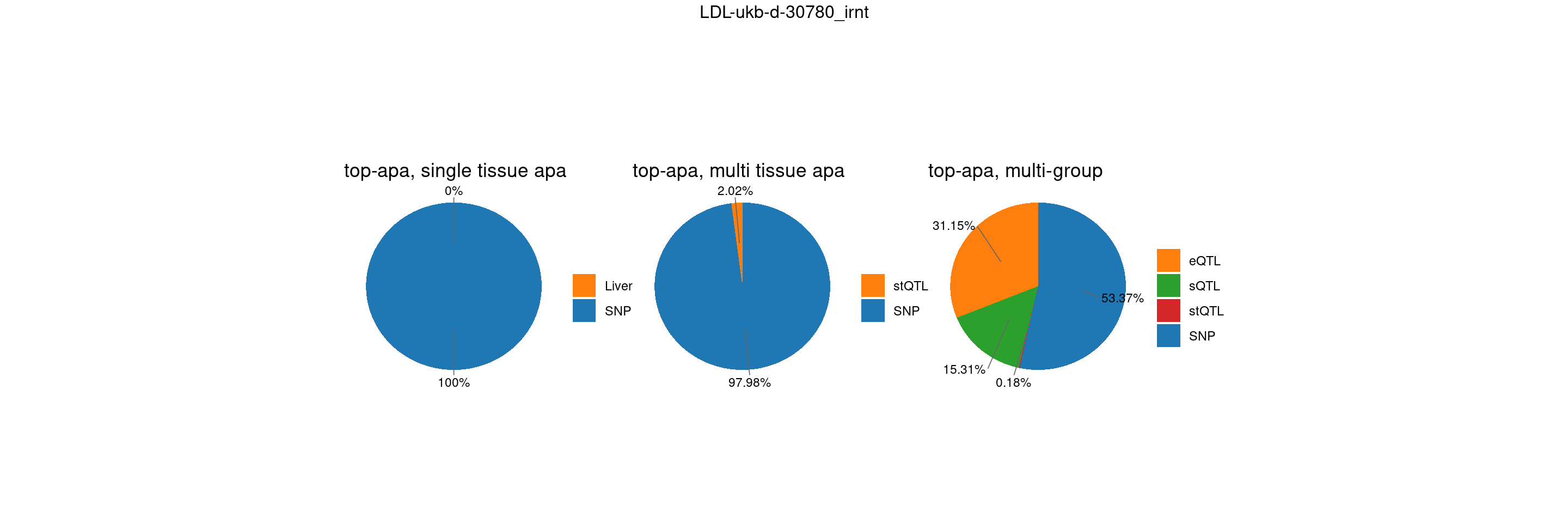
TableGrob (2 x 3) "arrange": 4 grobs
  z     cells    name                grob
1 1 (2-2,1-1) arrange      gtable[layout]
2 2 (2-2,2-2) arrange      gtable[layout]
3 3 (2-2,3-3) arrange      gtable[layout]
4 4 (1-1,1-3) arrange text[GRID.text.136]
param_susieST <- readRDS(paste0(folder_results_susieST_susie,"/",trait,"/",trait,".",st,".thin",thin,".",var_struc,".param.RDS"))
ctwas_parameters_susieST <- summarize_param(param_susieST, gwas_n)
total_nonSNPpve_susieST <- 1- ctwas_parameters_susieST$prop_heritability["SNP"]
pve_pie_by_type_susieST <- plot_piechart_topn(ctwas_parameters = ctwas_parameters_susieST, colors = colors, by = "type", title = "multi-group")
param_apaonly <- readRDS(paste0(folder_results_apaonly_susie,"/",trait,"/",trait,".",st,".thin",thin,".",var_struc,".param.RDS"))
ctwas_parameters_apaonly <- summarize_param(param_apaonly,gwas_n)
total_nonSNPpve_apaonly <- 1- ctwas_parameters_apaonly$prop_heritability["SNP"]
pve_pie_by_type_apaonly <- plot_piechart_topn(ctwas_parameters = ctwas_parameters_apaonly, colors = colors, by = "type", title = "multi tissue susie st")
top_tissue <- top_tissues[trait]
file_param_single <- paste0(folder_results_single_susie, trait, "/", trait, "_", top_tissue, ".thin", thin, ".", var_struc, ".param.RDS")
param_single <- readRDS(file_param_single)
ctwas_parameters_single <- summarize_param(param_single, gwas_n)
total_nonSNPpve_single <- 1- ctwas_parameters_single$prop_heritability["SNP"]
pve_pie_by_type_single <- plot_piechart_topn(ctwas_parameters = ctwas_parameters_single, colors = colors, by = "context", title = "single tissue susie st")
plot_multi(pve_pie_by_type_single,pve_pie_by_type_apaonly,pve_pie_by_type_susieST, title=trait)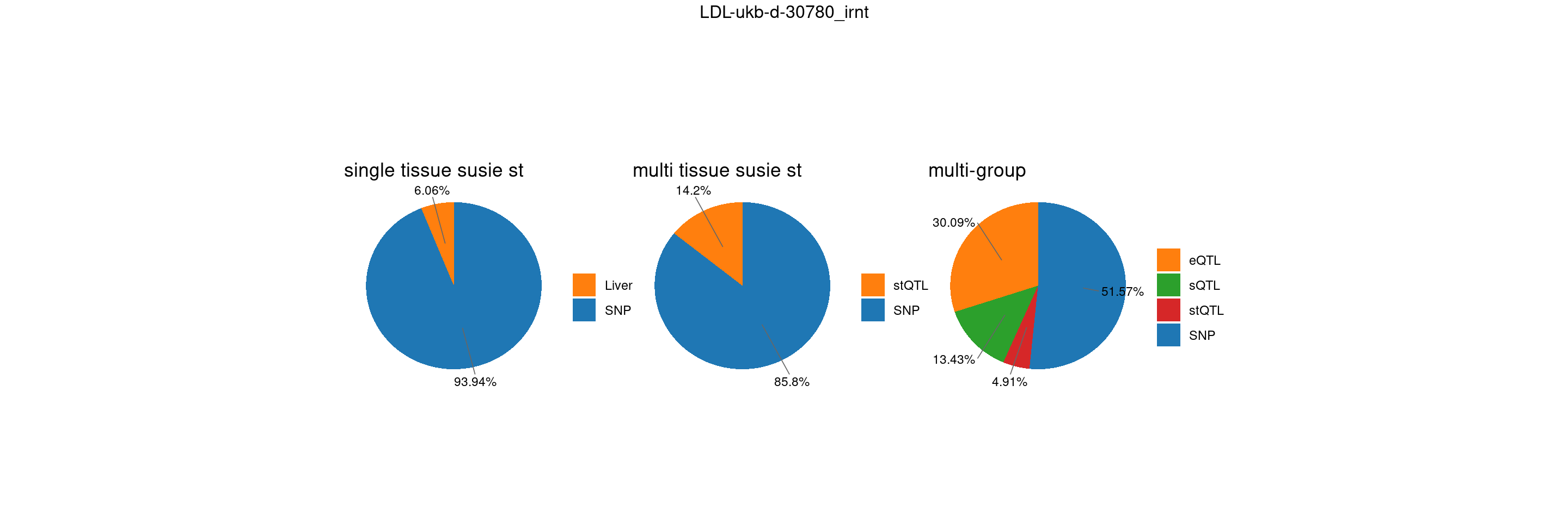
TableGrob (2 x 3) "arrange": 4 grobs
  z     cells    name                grob
1 1 (2-2,1-1) arrange      gtable[layout]
2 2 (2-2,2-2) arrange      gtable[layout]
3 3 (2-2,3-3) arrange      gtable[layout]
4 4 (1-1,1-3) arrange text[GRID.text.275]
IBD-ebi-a-GCST004131
trait <- "IBD-ebi-a-GCST004131"
st <- "with_susieST"

gwas_n <- samplesize[trait]
%h2g for setting: shared_all, thin = 1
thin <- 1
var_struc <- "shared_all"
param_susieST <- readRDS(paste0(folder_results_susieST,"/",trait,"/",trait,".",st,".thin",thin,".",var_struc,".param.RDS"))
ctwas_parameters_susieST <- summarize_param(param_susieST, gwas_n)
total_nonSNPpve_susieST <- 1- ctwas_parameters_susieST$prop_heritability["SNP"]
pve_pie_by_type_susieST <- plot_piechart_topn(ctwas_parameters = ctwas_parameters_susieST, colors = colors, by = "type", title = "top-apa, multi-group")
param_apaonly <- readRDS(paste0(folder_results_apaonly,"/",trait,"/",trait,".",st,".thin",thin,".",var_struc,".param.RDS"))
ctwas_parameters_apaonly <- summarize_param(param_apaonly,gwas_n)
total_nonSNPpve_apaonly <- 1- ctwas_parameters_apaonly$prop_heritability["SNP"]
pve_pie_by_type_apaonly <- plot_piechart_topn(ctwas_parameters = ctwas_parameters_apaonly, colors = colors, by = "type", title = "top-apa, multi tissue apa")
top_tissue <- top_tissues[trait]
file_param_single <- paste0(folder_results_single, trait, "/", trait, "_", top_tissue, ".thin", thin, ".", var_struc, ".param.RDS")
param_single <- readRDS(file_param_single)
ctwas_parameters_single <- summarize_param(param_single, gwas_n)
total_nonSNPpve_single <- 1- ctwas_parameters_single$prop_heritability["SNP"]
pve_pie_by_type_single <- plot_piechart_topn(ctwas_parameters = ctwas_parameters_single, colors = colors, by = "context", title = "top-apa, single tissue apa")
plot_multi(pve_pie_by_type_single,pve_pie_by_type_apaonly,pve_pie_by_type_susieST, title=trait)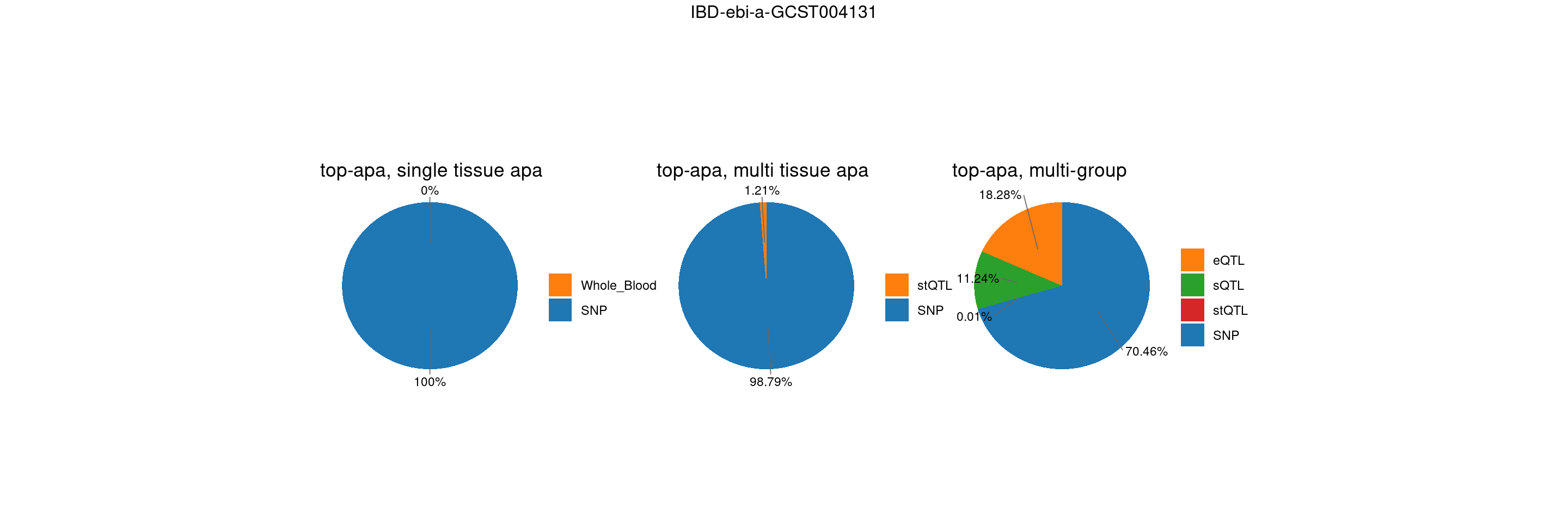
| Version | Author | Date |
|---|---|---|
| bda6e43 | XSun | 2025-04-09 |
TableGrob (2 x 3) "arrange": 4 grobs
  z     cells    name                grob
1 1 (2-2,1-1) arrange      gtable[layout]
2 2 (2-2,2-2) arrange      gtable[layout]
3 3 (2-2,3-3) arrange      gtable[layout]
4 4 (1-1,1-3) arrange text[GRID.text.414]
param_susieST <- readRDS(paste0(folder_results_susieST_susie,"/",trait,"/",trait,".",st,".thin",thin,".",var_struc,".param.RDS"))
ctwas_parameters_susieST <- summarize_param(param_susieST, gwas_n)
total_nonSNPpve_susieST <- 1- ctwas_parameters_susieST$prop_heritability["SNP"]
pve_pie_by_type_susieST <- plot_piechart_topn(ctwas_parameters = ctwas_parameters_susieST, colors = colors, by = "type", title = "multi-group")
param_apaonly <- readRDS(paste0(folder_results_apaonly_susie,"/",trait,"/",trait,".",st,".thin",thin,".",var_struc,".param.RDS"))
ctwas_parameters_apaonly <- summarize_param(param_apaonly,gwas_n)
total_nonSNPpve_apaonly <- 1- ctwas_parameters_apaonly$prop_heritability["SNP"]
pve_pie_by_type_apaonly <- plot_piechart_topn(ctwas_parameters = ctwas_parameters_apaonly, colors = colors, by = "type", title = "multi tissue susie st")
top_tissue <- top_tissues[trait]
file_param_single <- paste0(folder_results_single_susie, trait, "/", trait, "_", top_tissue, ".thin", thin, ".", var_struc, ".param.RDS")
param_single <- readRDS(file_param_single)
ctwas_parameters_single <- summarize_param(param_single, gwas_n)
total_nonSNPpve_single <- 1- ctwas_parameters_single$prop_heritability["SNP"]
pve_pie_by_type_single <- plot_piechart_topn(ctwas_parameters = ctwas_parameters_single, colors = colors, by = "context", title = "single tissue susie st")
plot_multi(pve_pie_by_type_single,pve_pie_by_type_apaonly,pve_pie_by_type_susieST, title=trait)
| Version | Author | Date |
|---|---|---|
| 6e49457 | XSun | 2025-04-17 |
TableGrob (2 x 3) "arrange": 4 grobs
  z     cells    name                grob
1 1 (2-2,1-1) arrange      gtable[layout]
2 2 (2-2,2-2) arrange      gtable[layout]
3 3 (2-2,3-3) arrange      gtable[layout]
4 4 (1-1,1-3) arrange text[GRID.text.553]
gene level results – whole blood
results_li <- read.table("/project/xinhe/xsun/multi_group_ctwas/16.apa_li_weights/data/IBD_genes_li.txt", header = T)

tissues_target <- c("Whole_Blood")
results_li_overlaptissue <- results_li[results_li$Tissue %in% tissues_target,]

ctwas_res <- readRDS("/project/xinhe/xsun/multi_group_ctwas/16.apa_li_weights/ctwas_output/apa//IBD-ebi-a-GCST004131/IBD-ebi-a-GCST004131_Whole_Blood.thin1.shared_all.L5.finemap_regions_res.RDS")

mapping_table <- readRDS("/project2/xinhe/shared_data/multigroup_ctwas/weights/mapping_files/apa_li.RDS")

susie_alpha_res <- ctwas_res$susie_alpha_res
susie_alpha_res$molecular_id <- sub("\\|[^|]*$", "", susie_alpha_res$id)
susie_alpha_res <- anno_susie_alpha_res(susie_alpha_res,
                                        mapping_table = mapping_table,
                                        map_by = "molecular_id",
                                        drop_unmapped = F)
2025-04-25 09:37:25 INFO::Annotating susie alpha result ...
2025-04-25 09:37:25 INFO::Map molecular traits to genessusie_alpha_res_uniq <- susie_alpha_res[!duplicated(susie_alpha_res$id),]
susie_summary <- susie_alpha_res_uniq %>%
group_by(gene_name) %>%
summarise(
susie_z = mean(z, na.rm = TRUE), # or median(z) if you prefer
susie_pip = max(susie_pip, na.rm = TRUE), # max to reflect strongest evidence
region_id = region_id,
id = id,
)
# Step 2: Merge with results_li
results_li_merged <- results_li_overlaptissue %>%
left_join(susie_summary, by = c("GeneName" = "gene_name"))
DT::datatable(results_li_merged,caption = htmltools::tags$caption( style = 'caption-side: left; text-align: left; color:black; font-size:150% ;',''),options = list(pageLength = 10) )results_li_merged <- results_li_merged[complete.cases(results_li_merged$region_id),]
weights <- readRDS("/project/xinhe/xsun/multi_group_ctwas/16.apa_li_weights/ctwas_output/apa//IBD-ebi-a-GCST004131/IBD-ebi-a-GCST004131_Whole_Blood.preprocessed.weights.ST.RDS")
snp_map <- readRDS("/project2/xinhe/shared_data/multigroup_ctwas/LD_region_info/snp_map.RDS")
finemap_res <- ctwas_res$finemap_res
finemap_res$molecular_id <- get_molecular_ids(finemap_res)
finemap_res <- anno_finemap_res(finemap_res,
snp_map = snp_map,
mapping_table = mapping_table,
add_gene_annot = TRUE,
map_by = "molecular_id",
drop_unmapped = TRUE,
add_position = TRUE,
use_gene_pos = "mid")2025-04-25 09:37:43 INFO::Annotating fine-mapping result ...
2025-04-25 09:37:45 INFO::Map molecular traits to genes
2025-04-25 09:37:45 INFO::Drop 966 unmapped molecular traits
2025-04-25 09:38:00 INFO::Add gene positions
2025-04-25 09:38:00 INFO::Add SNP positionsfor (i in 1:nrow(results_li_merged)) {
region_id <- results_li_merged$region_id[i]
p <- make_locusplot(finemap_res,
region_id = region_id,
ens_db = ens_db,
weights = weights,
highlight_pip = 0.8,
filter_protein_coding_genes = TRUE,
filter_cs = F,
focal_id = results_li_merged$id[i],
color_pval_by = "cs",
color_pip_by = "cs")
print(p)
}2025-04-25 09:38:11 INFO::Limit to protein coding genes
2025-04-25 09:38:11 INFO::focal id: NM_181698|CCNY|chr10|+|Whole_Blood_stQTL
2025-04-25 09:38:11 INFO::focal molecular trait:
2025-04-25 09:38:11 INFO::Range of locus: chr10:34820327-36282921
2025-04-25 09:38:12 INFO::focal molecular trait QTL positions: 35456424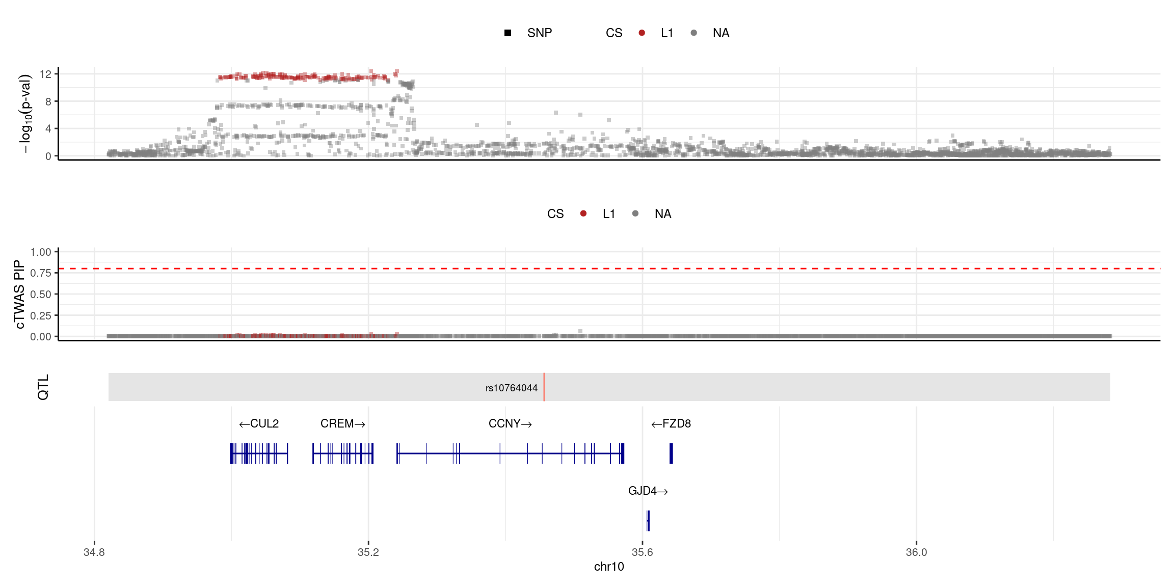
2025-04-25 09:38:12 INFO::Limit to protein coding genes
2025-04-25 09:38:12 INFO::focal id: NM_005253|FOSL2|chr2|+|Whole_Blood_stQTL
2025-04-25 09:38:12 INFO::focal molecular trait:
2025-04-25 09:38:12 INFO::Range of locus: chr2:28376782-28994103
2025-04-25 09:38:13 INFO::focal molecular trait QTL positions: 28412873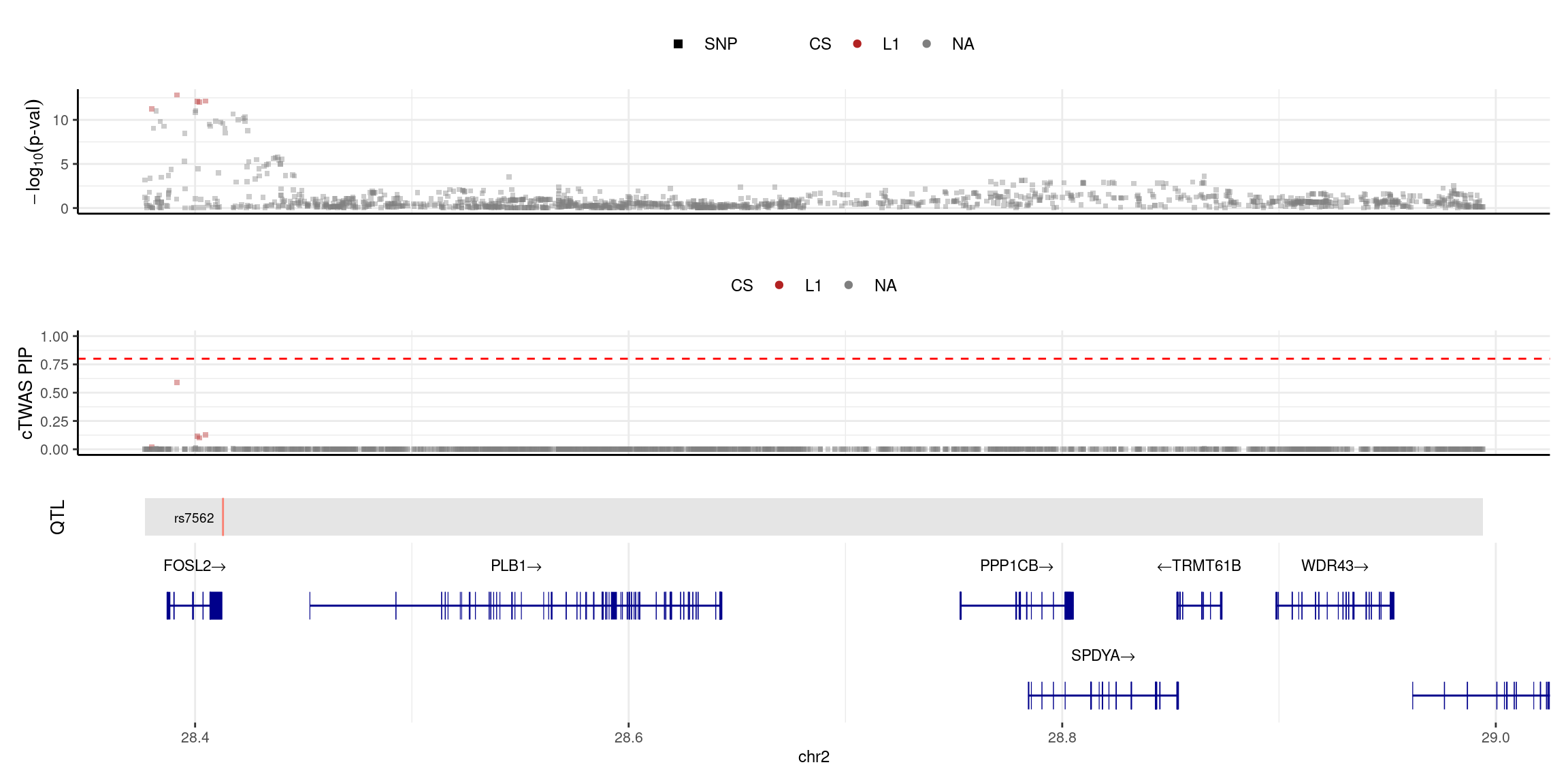
2025-04-25 09:38:14 INFO::Limit to protein coding genes
2025-04-25 09:38:14 INFO::focal id: NM_022349|MS4A6A|chr11|-|Whole_Blood_stQTL
2025-04-25 09:38:14 INFO::focal molecular trait:
2025-04-25 09:38:14 INFO::Range of locus: chr11:59012976-62455196
2025-04-25 09:38:14 INFO::focal molecular trait QTL positions: 60200909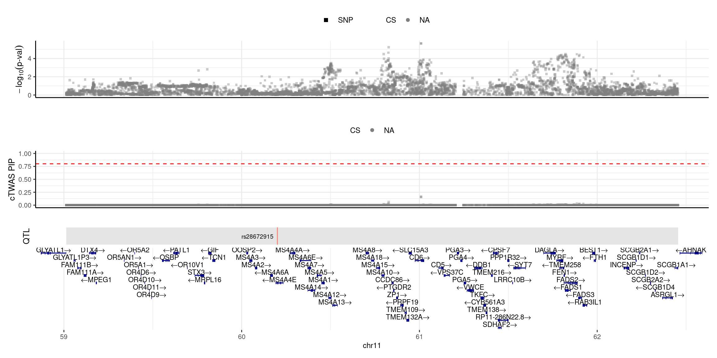
2025-04-25 09:38:16 INFO::Limit to protein coding genes
2025-04-25 09:38:16 INFO::focal id: NM_152851|MS4A6A|chr11|-|Whole_Blood_stQTL
2025-04-25 09:38:16 INFO::focal molecular trait:
2025-04-25 09:38:16 INFO::Range of locus: chr11:59012976-62455196
2025-04-25 09:38:16 INFO::focal molecular trait QTL positions: 60088555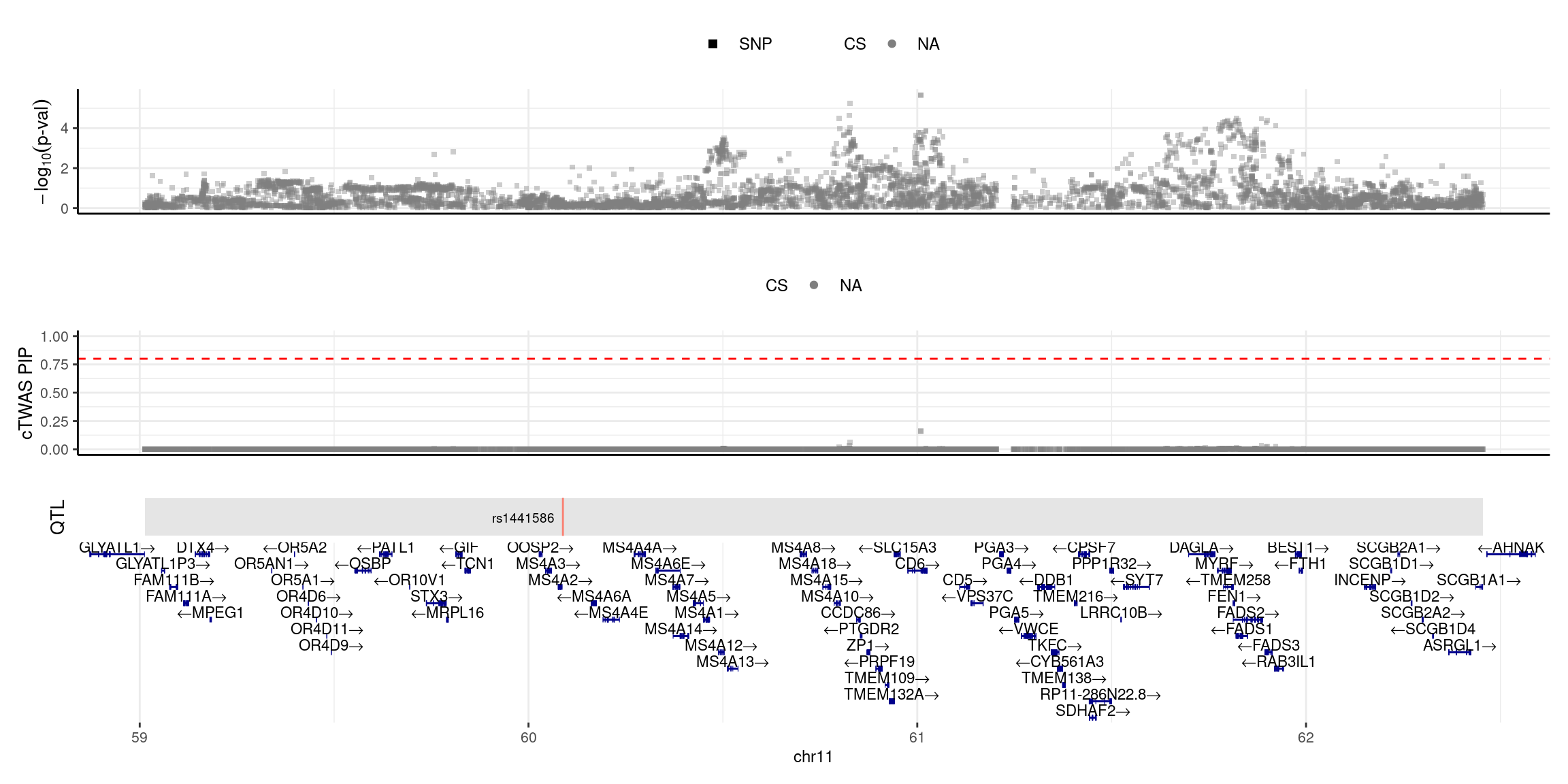
2025-04-25 09:38:19 INFO::Limit to protein coding genes
2025-04-25 09:38:19 INFO::focal id: NM_177939|P4HTM|chr3|+|Whole_Blood_stQTL
2025-04-25 09:38:19 INFO::focal molecular trait:
2025-04-25 09:38:19 INFO::Range of locus: chr3:49279805-51794719
2025-04-25 09:38:19 INFO::focal molecular trait QTL positions: 49970685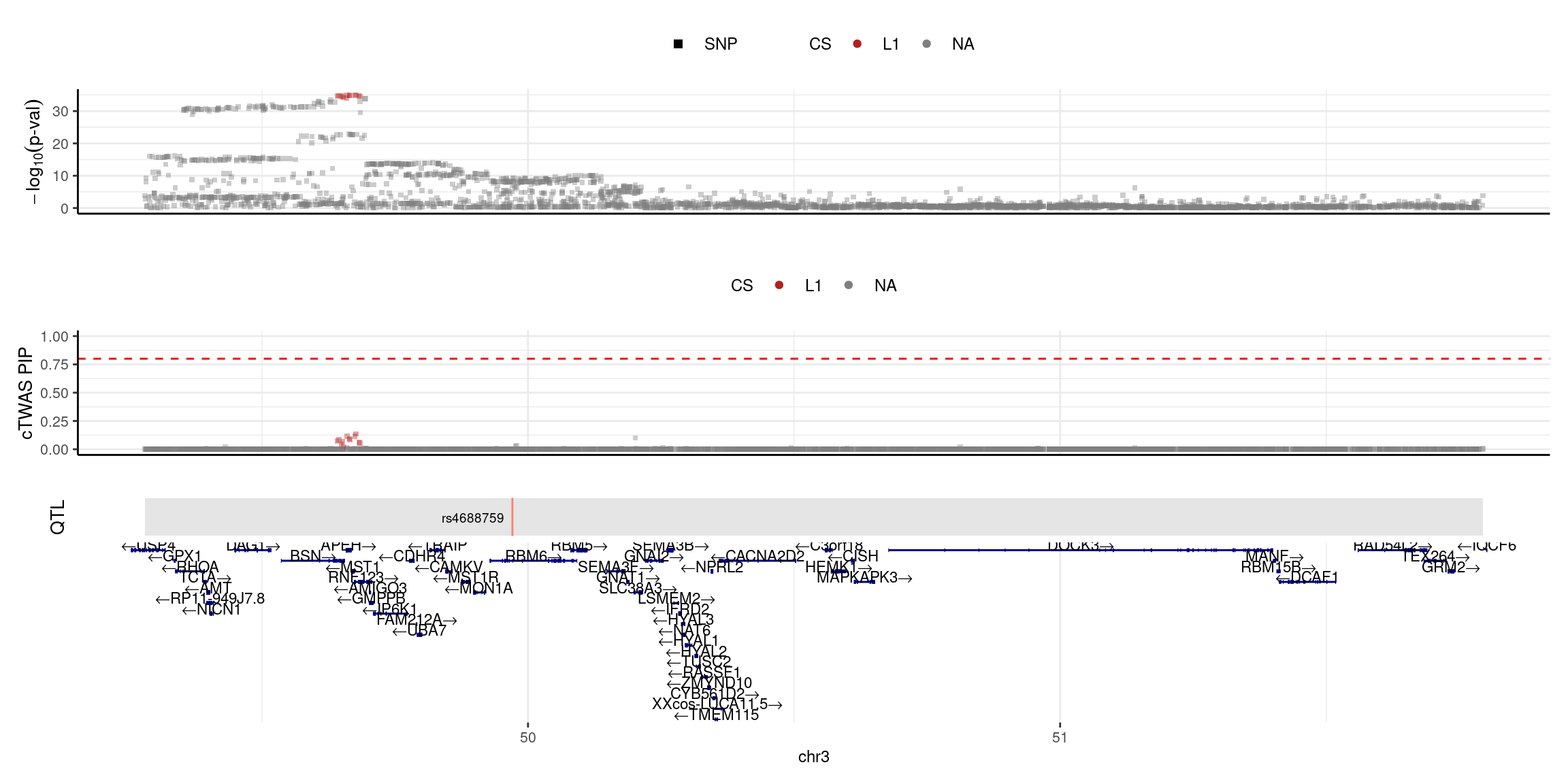
2025-04-25 09:38:20 INFO::Limit to protein coding genes
2025-04-25 09:38:20 INFO::focal id: NM_053055|THEM4|chr1|-|Whole_Blood_stQTL
2025-04-25 09:38:20 INFO::focal molecular trait:
2025-04-25 09:38:20 INFO::Range of locus: chr1:151566589-153207547
2025-04-25 09:38:20 INFO::focal molecular trait QTL positions: 151865616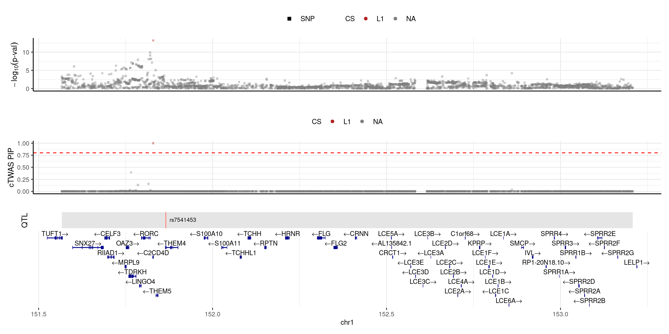
T2D-panukb
trait <- "T2D-panukb"
st <- "with_susieST"

gwas_n <- samplesize[trait]
%h2g for setting: shared_all, thin = 1
thin <- 1
var_struc <- "shared_all"
param_susieST <- readRDS(paste0(folder_results_susieST,"/",trait,"/",trait,".",st,".thin",thin,".",var_struc,".param.RDS"))
ctwas_parameters_susieST <- summarize_param(param_susieST, gwas_n)
total_nonSNPpve_susieST <- 1- ctwas_parameters_susieST$prop_heritability["SNP"]
pve_pie_by_type_susieST <- plot_piechart_topn(ctwas_parameters = ctwas_parameters_susieST, colors = colors, by = "type", title = "top-apa, multi-group")
param_apaonly <- readRDS(paste0(folder_results_apaonly,"/",trait,"/",trait,".",st,".thin",thin,".",var_struc,".param.RDS"))
ctwas_parameters_apaonly <- summarize_param(param_apaonly,gwas_n)
total_nonSNPpve_apaonly <- 1- ctwas_parameters_apaonly$prop_heritability["SNP"]
pve_pie_by_type_apaonly <- plot_piechart_topn(ctwas_parameters = ctwas_parameters_apaonly, colors = colors, by = "type", title = "top-apa, multi tissue apa")
top_tissue <- top_tissues[trait]
file_param_single <- paste0(folder_results_single, trait, "/", trait, "_", top_tissue, ".thin", thin, ".", var_struc, ".param.RDS")
param_single <- readRDS(file_param_single)
ctwas_parameters_single <- summarize_param(param_single, gwas_n)
total_nonSNPpve_single <- 1- ctwas_parameters_single$prop_heritability["SNP"]
pve_pie_by_type_single <- plot_piechart_topn(ctwas_parameters = ctwas_parameters_single, colors = colors, by = "context", title = "top-apa, single tissue apa")
plot_multi(pve_pie_by_type_single,pve_pie_by_type_apaonly,pve_pie_by_type_susieST, title=trait)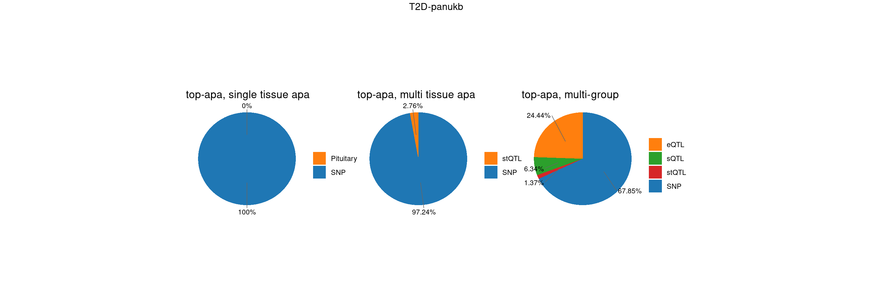
| Version | Author | Date |
|---|---|---|
| 278bbd9 | XSun | 2025-04-17 |
TableGrob (2 x 3) "arrange": 4 grobs
  z     cells    name                 grob
1 1 (2-2,1-1) arrange       gtable[layout]
2 2 (2-2,2-2) arrange       gtable[layout]
3 3 (2-2,3-3) arrange       gtable[layout]
4 4 (1-1,1-3) arrange text[GRID.text.2032]
param_susieST <- readRDS(paste0(folder_results_susieST_susie,"/",trait,"/",trait,".",st,".thin",thin,".",var_struc,".param.RDS"))
ctwas_parameters_susieST <- summarize_param(param_susieST, gwas_n)
total_nonSNPpve_susieST <- 1- ctwas_parameters_susieST$prop_heritability["SNP"]
pve_pie_by_type_susieST <- plot_piechart_topn(ctwas_parameters = ctwas_parameters_susieST, colors = colors, by = "type", title = "multi-group")
param_apaonly <- readRDS(paste0(folder_results_apaonly_susie,"/",trait,"/",trait,".",st,".thin",thin,".",var_struc,".param.RDS"))
ctwas_parameters_apaonly <- summarize_param(param_apaonly,gwas_n)
total_nonSNPpve_apaonly <- 1- ctwas_parameters_apaonly$prop_heritability["SNP"]
pve_pie_by_type_apaonly <- plot_piechart_topn(ctwas_parameters = ctwas_parameters_apaonly, colors = colors, by = "type", title = "multi tissue susie st")
top_tissue <- top_tissues[trait]
file_param_single <- paste0(folder_results_single_susie, trait, "/", trait, "_", top_tissue, ".thin", thin, ".", var_struc, ".param.RDS")
param_single <- readRDS(file_param_single)
ctwas_parameters_single <- summarize_param(param_single, gwas_n)
total_nonSNPpve_single <- 1- ctwas_parameters_single$prop_heritability["SNP"]
pve_pie_by_type_single <- plot_piechart_topn(ctwas_parameters = ctwas_parameters_single, colors = colors, by = "context", title = "single tissue susie st")
plot_multi(pve_pie_by_type_single,pve_pie_by_type_apaonly,pve_pie_by_type_susieST, title=trait)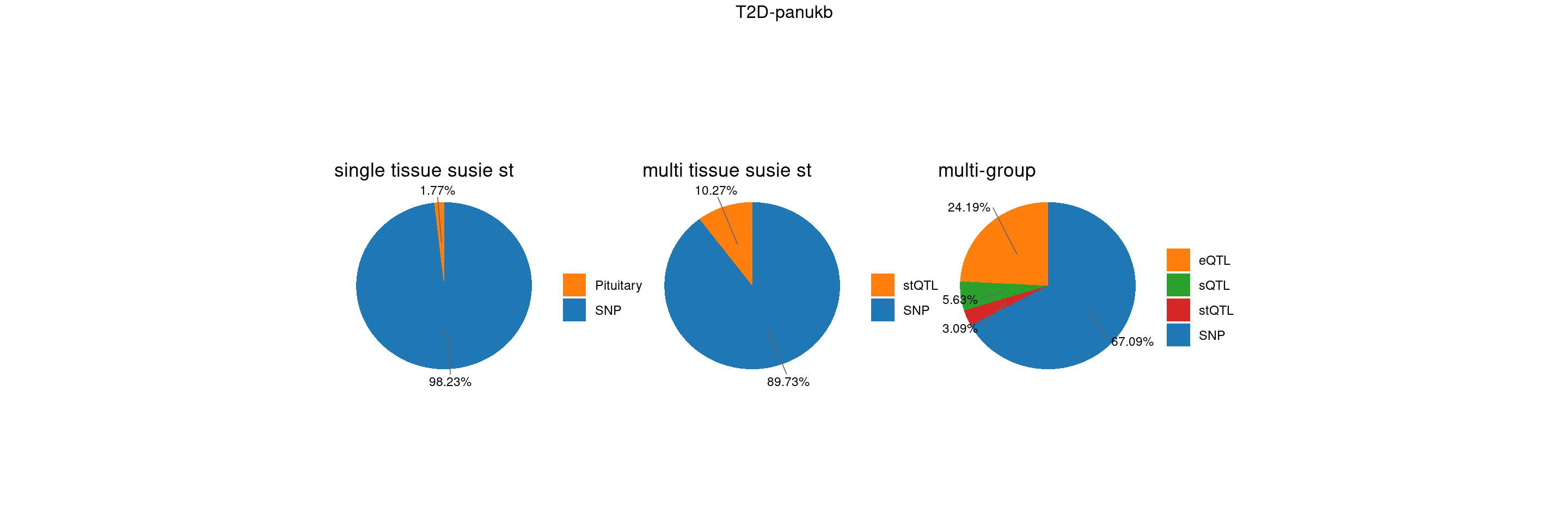
| Version | Author | Date |
|---|---|---|
| bda6e43 | XSun | 2025-04-09 |
TableGrob (2 x 3) "arrange": 4 grobs
  z     cells    name                 grob
1 1 (2-2,1-1) arrange       gtable[layout]
2 2 (2-2,2-2) arrange       gtable[layout]
3 3 (2-2,3-3) arrange       gtable[layout]
4 4 (1-1,1-3) arrange text[GRID.text.2171]
BMI-panukb
trait <- "BMI-panukb"
st <- "with_susieST"

gwas_n <- samplesize[trait]
%h2g for setting: shared_all, thin = 1
thin <- 1
var_struc <- "shared_all"
param_susieST <- readRDS(paste0(folder_results_susieST,"/",trait,"/",trait,".",st,".thin",thin,".",var_struc,".param.RDS"))
ctwas_parameters_susieST <- summarize_param(param_susieST, gwas_n)
total_nonSNPpve_susieST <- 1- ctwas_parameters_susieST$prop_heritability["SNP"]
pve_pie_by_type_susieST <- plot_piechart_topn(ctwas_parameters = ctwas_parameters_susieST, colors = colors, by = "type", title = "top-apa, multi-group")
param_apaonly <- readRDS(paste0(folder_results_apaonly,"/",trait,"/",trait,".",st,".thin",thin,".",var_struc,".param.RDS"))
ctwas_parameters_apaonly <- summarize_param(param_apaonly,gwas_n)
total_nonSNPpve_apaonly <- 1- ctwas_parameters_apaonly$prop_heritability["SNP"]
pve_pie_by_type_apaonly <- plot_piechart_topn(ctwas_parameters = ctwas_parameters_apaonly, colors = colors, by = "type", title = "top-apa, multi tissue apa")
top_tissue <- top_tissues[trait]
file_param_single <- paste0(folder_results_single, trait, "/", trait, "_", top_tissue, ".thin", thin, ".", var_struc, ".param.RDS")
param_single <- readRDS(file_param_single)
ctwas_parameters_single <- summarize_param(param_single, gwas_n)
total_nonSNPpve_single <- 1- ctwas_parameters_single$prop_heritability["SNP"]
pve_pie_by_type_single <- plot_piechart_topn(ctwas_parameters = ctwas_parameters_single, colors = colors, by = "context", title = "top-apa, single tissue apa")
plot_multi(pve_pie_by_type_single,pve_pie_by_type_apaonly,pve_pie_by_type_susieST, title=trait)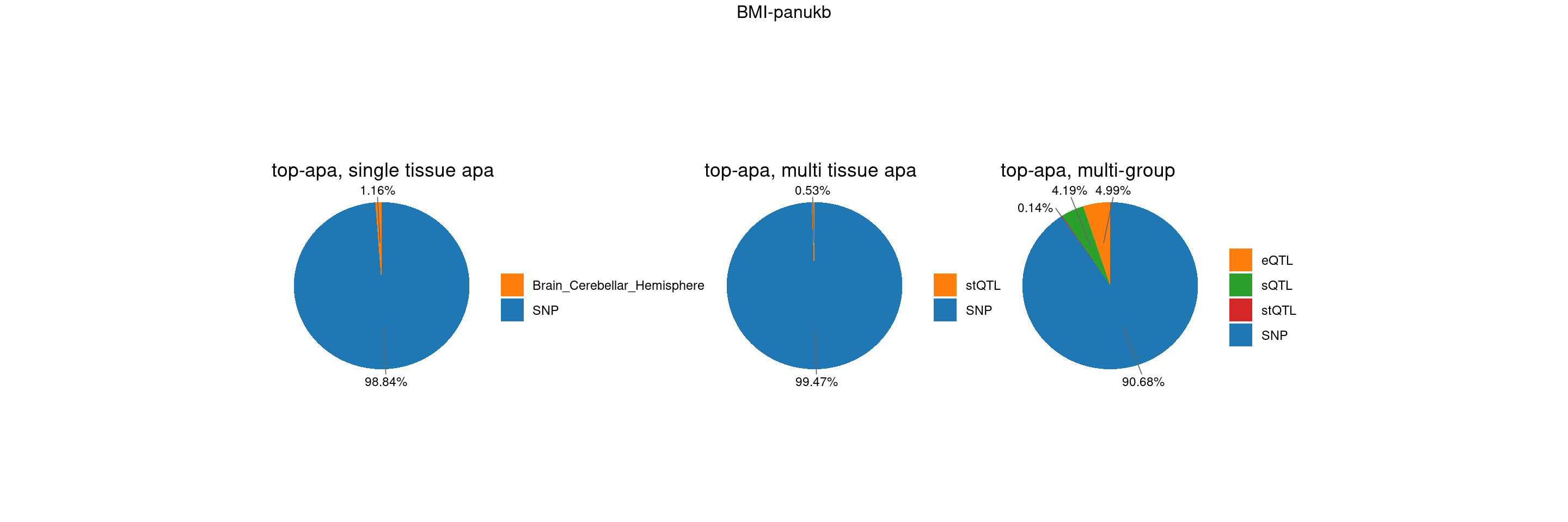
TableGrob (2 x 3) "arrange": 4 grobs
  z     cells    name                 grob
1 1 (2-2,1-1) arrange       gtable[layout]
2 2 (2-2,2-2) arrange       gtable[layout]
3 3 (2-2,3-3) arrange       gtable[layout]
4 4 (1-1,1-3) arrange text[GRID.text.2310]
param_susieST <- readRDS(paste0(folder_results_susieST_susie,"/",trait,"/",trait,".",st,".thin",thin,".",var_struc,".param.RDS"))
ctwas_parameters_susieST <- summarize_param(param_susieST, gwas_n)
total_nonSNPpve_susieST <- 1- ctwas_parameters_susieST$prop_heritability["SNP"]
pve_pie_by_type_susieST <- plot_piechart_topn(ctwas_parameters = ctwas_parameters_susieST, colors = colors, by = "type", title = "multi-group")
param_apaonly <- readRDS(paste0(folder_results_apaonly_susie,"/",trait,"/",trait,".",st,".thin",thin,".",var_struc,".param.RDS"))
ctwas_parameters_apaonly <- summarize_param(param_apaonly,gwas_n)
total_nonSNPpve_apaonly <- 1- ctwas_parameters_apaonly$prop_heritability["SNP"]
pve_pie_by_type_apaonly <- plot_piechart_topn(ctwas_parameters = ctwas_parameters_apaonly, colors = colors, by = "type", title = "multi tissue susie st")
top_tissue <- top_tissues[trait]
file_param_single <- paste0(folder_results_single_susie, trait, "/", trait, "_", top_tissue, ".thin", thin, ".", var_struc, ".param.RDS")
param_single <- readRDS(file_param_single)
ctwas_parameters_single <- summarize_param(param_single, gwas_n)
total_nonSNPpve_single <- 1- ctwas_parameters_single$prop_heritability["SNP"]
pve_pie_by_type_single <- plot_piechart_topn(ctwas_parameters = ctwas_parameters_single, colors = colors, by = "context", title = "single tissue susie st")
plot_multi(pve_pie_by_type_single,pve_pie_by_type_apaonly,pve_pie_by_type_susieST, title=trait)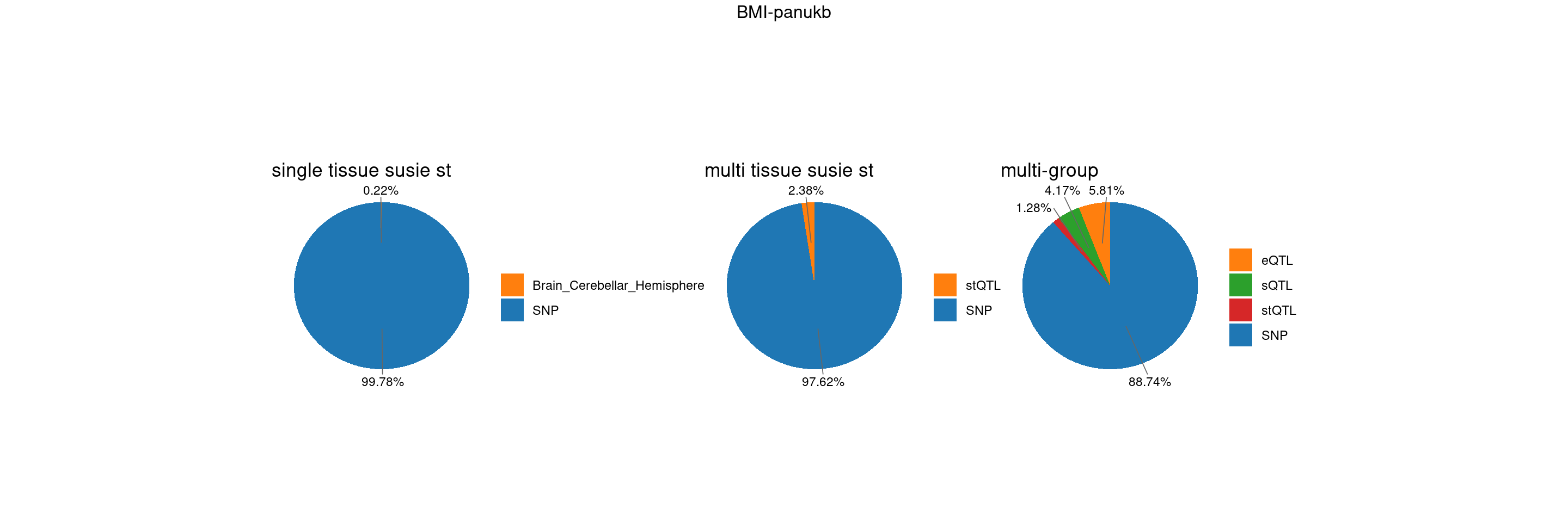
TableGrob (2 x 3) "arrange": 4 grobs
  z     cells    name                 grob
1 1 (2-2,1-1) arrange       gtable[layout]
2 2 (2-2,2-2) arrange       gtable[layout]
3 3 (2-2,3-3) arrange       gtable[layout]
4 4 (1-1,1-3) arrange text[GRID.text.2449]
RBC-panukb
trait <- "RBC-panukb"
st <- "with_susieST"

gwas_n <- samplesize[trait]
%h2g for setting: shared_all, thin = 1
thin <- 1
var_struc <- "shared_all"
param_susieST <- readRDS(paste0(folder_results_susieST,"/",trait,"/",trait,".",st,".thin",thin,".",var_struc,".param.RDS"))
ctwas_parameters_susieST <- summarize_param(param_susieST, gwas_n)
total_nonSNPpve_susieST <- 1- ctwas_parameters_susieST$prop_heritability["SNP"]
pve_pie_by_type_susieST <- plot_piechart_topn(ctwas_parameters = ctwas_parameters_susieST, colors = colors, by = "type", title = "top-apa, multi-group")
param_apaonly <- readRDS(paste0(folder_results_apaonly,"/",trait,"/",trait,".",st,".thin",thin,".",var_struc,".param.RDS"))
ctwas_parameters_apaonly <- summarize_param(param_apaonly,gwas_n)
total_nonSNPpve_apaonly <- 1- ctwas_parameters_apaonly$prop_heritability["SNP"]
pve_pie_by_type_apaonly <- plot_piechart_topn(ctwas_parameters = ctwas_parameters_apaonly, colors = colors, by = "type", title = "top-apa, multi tissue apa")
top_tissue <- top_tissues[trait]
file_param_single <- paste0(folder_results_single, trait, "/", trait, "_", top_tissue, ".thin", thin, ".", var_struc, ".param.RDS")
param_single <- readRDS(file_param_single)
ctwas_parameters_single <- summarize_param(param_single, gwas_n)
total_nonSNPpve_single <- 1- ctwas_parameters_single$prop_heritability["SNP"]
pve_pie_by_type_single <- plot_piechart_topn(ctwas_parameters = ctwas_parameters_single, colors = colors, by = "context", title = "top-apa, single tissue apa")
plot_multi(pve_pie_by_type_single,pve_pie_by_type_apaonly,pve_pie_by_type_susieST, title=trait)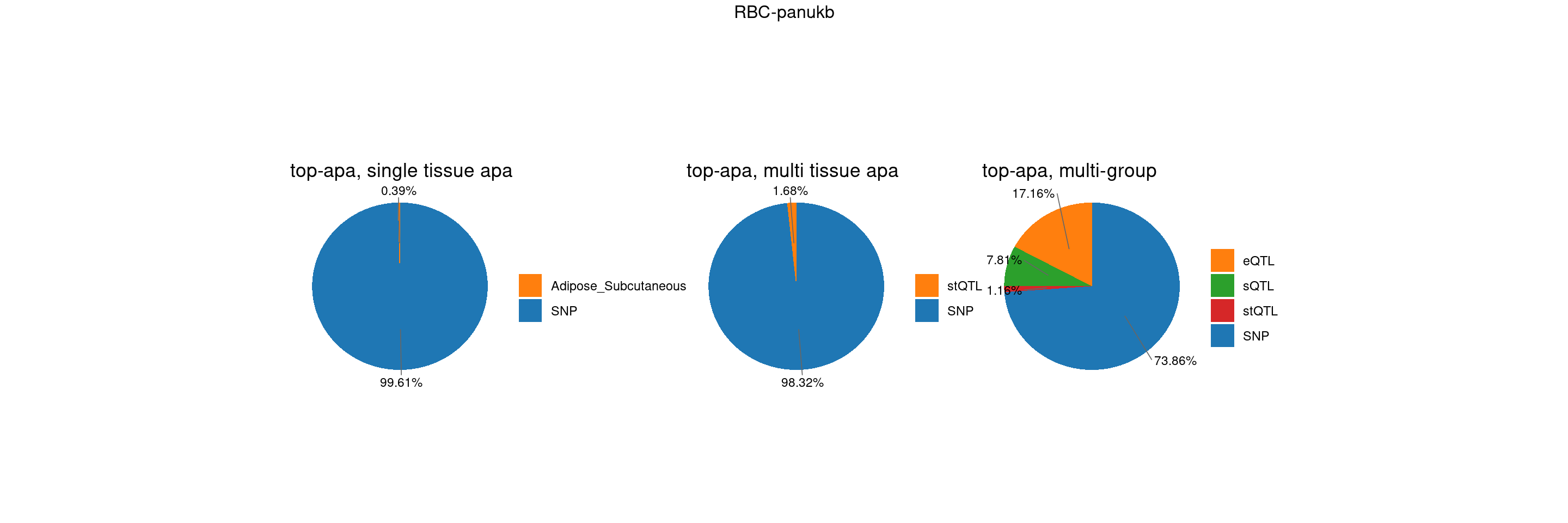
TableGrob (2 x 3) "arrange": 4 grobs
  z     cells    name                 grob
1 1 (2-2,1-1) arrange       gtable[layout]
2 2 (2-2,2-2) arrange       gtable[layout]
3 3 (2-2,3-3) arrange       gtable[layout]
4 4 (1-1,1-3) arrange text[GRID.text.2588]
param_susieST <- readRDS(paste0(folder_results_susieST_susie,"/",trait,"/",trait,".",st,".thin",thin,".",var_struc,".param.RDS"))
ctwas_parameters_susieST <- summarize_param(param_susieST, gwas_n)
total_nonSNPpve_susieST <- 1- ctwas_parameters_susieST$prop_heritability["SNP"]
pve_pie_by_type_susieST <- plot_piechart_topn(ctwas_parameters = ctwas_parameters_susieST, colors = colors, by = "type", title = "multi-group")
param_apaonly <- readRDS(paste0(folder_results_apaonly_susie,"/",trait,"/",trait,".",st,".thin",thin,".",var_struc,".param.RDS"))
ctwas_parameters_apaonly <- summarize_param(param_apaonly,gwas_n)
total_nonSNPpve_apaonly <- 1- ctwas_parameters_apaonly$prop_heritability["SNP"]
pve_pie_by_type_apaonly <- plot_piechart_topn(ctwas_parameters = ctwas_parameters_apaonly, colors = colors, by = "type", title = "multi tissue susie st")
top_tissue <- top_tissues[trait]
file_param_single <- paste0(folder_results_single_susie, trait, "/", trait, "_", top_tissue, ".thin", thin, ".", var_struc, ".param.RDS")
param_single <- readRDS(file_param_single)
ctwas_parameters_single <- summarize_param(param_single, gwas_n)
total_nonSNPpve_single <- 1- ctwas_parameters_single$prop_heritability["SNP"]
pve_pie_by_type_single <- plot_piechart_topn(ctwas_parameters = ctwas_parameters_single, colors = colors, by = "context", title = "single tissue susie st")
plot_multi(pve_pie_by_type_single,pve_pie_by_type_apaonly,pve_pie_by_type_susieST, title=trait)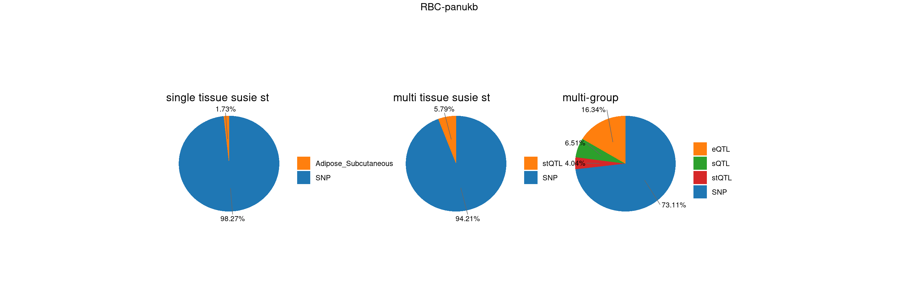
| Version | Author | Date |
|---|---|---|
| bda6e43 | XSun | 2025-04-09 |
TableGrob (2 x 3) "arrange": 4 grobs
  z     cells    name                 grob
1 1 (2-2,1-1) arrange       gtable[layout]
2 2 (2-2,2-2) arrange       gtable[layout]
3 3 (2-2,3-3) arrange       gtable[layout]
4 4 (1-1,1-3) arrange text[GRID.text.2727]
sessionInfo()R version 4.2.0 (2022-04-22)
Platform: x86_64-pc-linux-gnu (64-bit)
Running under: CentOS Linux 7 (Core)
Matrix products: default
BLAS/LAPACK: /software/openblas-0.3.13-el7-x86_64/lib/libopenblas_haswellp-r0.3.13.so
locale:
[1] C
attached base packages:
[1] grid stats4 stats graphics grDevices utils datasets
[8] methods base
other attached packages:
[1] egg_0.4.5 gridExtra_2.3
[3] ggrepel_0.9.1 pheatmap_1.0.12
[5] EnsDb.Hsapiens.v86_2.99.0 ensembldb_2.20.2
[7] AnnotationFilter_1.20.0 GenomicFeatures_1.48.3
[9] AnnotationDbi_1.58.0 Biobase_2.56.0
[11] GenomicRanges_1.48.0 GenomeInfoDb_1.39.9
[13] IRanges_2.30.0 S4Vectors_0.34.0
[15] BiocGenerics_0.42.0 forcats_0.5.1
[17] stringr_1.5.1 dplyr_1.1.4
[19] purrr_1.0.2 readr_2.1.2
[21] tidyr_1.3.0 tibble_3.2.1
[23] tidyverse_1.3.1 ggplot2_3.5.1
[25] ctwas_0.5.4.9000
loaded via a namespace (and not attached):
[1] readxl_1.4.0 backports_1.4.1
[3] workflowr_1.7.0 BiocFileCache_2.4.0
[5] repr_1.1.4 lazyeval_0.2.2
[7] crosstalk_1.2.0 BiocParallel_1.30.3
[9] LDlinkR_1.2.3 digest_0.6.29
[11] htmltools_0.5.2 fansi_1.0.3
[13] magrittr_2.0.3 memoise_2.0.1
[15] tzdb_0.4.0 Biostrings_2.64.0
[17] modelr_0.1.8 AMR_2.1.1
[19] matrixStats_0.62.0 locuszoomr_0.2.1
[21] prettyunits_1.1.1 colorspace_2.0-3
[23] skimr_2.1.4 blob_1.2.3
[25] rvest_1.0.2 rappdirs_0.3.3
[27] haven_2.5.0 xfun_0.41
[29] crayon_1.5.1 RCurl_1.98-1.7
[31] jsonlite_1.8.0 zoo_1.8-10
[33] glue_1.6.2 gtable_0.3.0
[35] zlibbioc_1.42.0 XVector_0.36.0
[37] DelayedArray_0.22.0 scales_1.3.0
[39] DBI_1.2.2 Rcpp_1.0.12
[41] viridisLite_0.4.0 progress_1.2.2
[43] bit_4.0.4 DT_0.22
[45] htmlwidgets_1.5.4 httr_1.4.3
[47] RColorBrewer_1.1-3 ellipsis_0.3.2
[49] farver_2.1.0 pkgconfig_2.0.3
[51] XML_3.99-0.14 sass_0.4.1
[53] dbplyr_2.1.1 utf8_1.2.2
[55] labeling_0.4.2 tidyselect_1.2.0
[57] rlang_1.1.2 later_1.3.0
[59] munsell_0.5.0 pgenlibr_0.3.3
[61] cellranger_1.1.0 tools_4.2.0
[63] cachem_1.0.6 cli_3.6.1
[65] generics_0.1.2 RSQLite_2.3.1
[67] broom_0.8.0 evaluate_0.15
[69] fastmap_1.1.0 yaml_2.3.5
[71] knitr_1.39 bit64_4.0.5
[73] fs_1.5.2 KEGGREST_1.36.3
[75] whisker_0.4 xml2_1.3.3
[77] biomaRt_2.54.1 compiler_4.2.0
[79] rstudioapi_0.13 plotly_4.10.0
[81] filelock_1.0.2 curl_4.3.2
[83] png_0.1-7 reprex_2.0.1
[85] bslib_0.3.1 stringi_1.7.6
[87] highr_0.9 lattice_0.20-45
[89] ProtGenerics_1.28.0 Matrix_1.5-3
[91] vctrs_0.6.5 pillar_1.9.0
[93] lifecycle_1.0.4 jquerylib_0.1.4
[95] data.table_1.14.2 cowplot_1.1.1
[97] bitops_1.0-7 irlba_2.3.5
[99] httpuv_1.6.5 rtracklayer_1.56.0
[101] R6_2.5.1 BiocIO_1.6.0
[103] promises_1.2.0.1 codetools_0.2-18
[105] assertthat_0.2.1 SummarizedExperiment_1.26.1
[107] rprojroot_2.0.3 rjson_0.2.21
[109] withr_2.5.0 GenomicAlignments_1.32.0
[111] Rsamtools_2.12.0 GenomeInfoDbData_1.2.8
[113] parallel_4.2.0 hms_1.1.1
[115] gggrid_0.2-0 rmarkdown_2.25
[117] MatrixGenerics_1.8.0 logging_0.10-108
[119] git2r_0.30.1 mixsqp_0.3-43
[121] lubridate_1.8.0 base64enc_0.1-3
[123] restfulr_0.0.14