Comparing predictdb & Munro: predictdb eQTL + sQTL VS Munro 6 modalities
XSun
2024-08-08
Last updated: 2024-09-12
Checks: 6 1
Knit directory: multigroup_ctwas_analysis/
This reproducible R Markdown analysis was created with workflowr (version 1.7.0). The Checks tab describes the reproducibility checks that were applied when the results were created. The Past versions tab lists the development history.
The R Markdown file has unstaged changes. To know which version of
the R Markdown file created these results, you’ll want to first commit
it to the Git repo. If you’re still working on the analysis, you can
ignore this warning. When you’re finished, you can run
wflow_publish to commit the R Markdown file and build the
HTML.
Great job! The global environment was empty. Objects defined in the global environment can affect the analysis in your R Markdown file in unknown ways. For reproduciblity it’s best to always run the code in an empty environment.
The command set.seed(20231112) was run prior to running
the code in the R Markdown file. Setting a seed ensures that any results
that rely on randomness, e.g. subsampling or permutations, are
reproducible.
Great job! Recording the operating system, R version, and package versions is critical for reproducibility.
Nice! There were no cached chunks for this analysis, so you can be confident that you successfully produced the results during this run.
Great job! Using relative paths to the files within your workflowr project makes it easier to run your code on other machines.
Great! You are using Git for version control. Tracking code development and connecting the code version to the results is critical for reproducibility.
The results in this page were generated with repository version 525859b. See the Past versions tab to see a history of the changes made to the R Markdown and HTML files.
Note that you need to be careful to ensure that all relevant files for
the analysis have been committed to Git prior to generating the results
(you can use wflow_publish or
wflow_git_commit). workflowr only checks the R Markdown
file, but you know if there are other scripts or data files that it
depends on. Below is the status of the Git repository when the results
were generated:
Ignored files:
    Ignored:    .Rhistory
    Ignored:    results/

Unstaged changes:
    Modified:   analysis/multi_group_compare_predictdb_munro_4weights_8weights.Rmd
    Modified:   analysis/multi_group_compare_predictdb_munro_updated.Rmd
Note that any generated files, e.g. HTML, png, CSS, etc., are not included in this status report because it is ok for generated content to have uncommitted changes.
These are the previous versions of the repository in which changes were
made to the R Markdown
(analysis/multi_group_compare_predictdb_munro_updated.Rmd)
and HTML
(docs/multi_group_compare_predictdb_munro_updated.html)
files. If you’ve configured a remote Git repository (see
?wflow_git_remote), click on the hyperlinks in the table
below to view the files as they were in that past version.
| File | Version | Author | Date | Message |
|---|---|---|---|---|
| Rmd | 525859b | XSun | 2024-09-10 | update |
| html | 525859b | XSun | 2024-09-10 | update |
| Rmd | d45c3aa | XSun | 2024-09-09 | update |
| html | d45c3aa | XSun | 2024-09-09 | update |
| Rmd | a581199 | XSun | 2024-09-09 | update |
| html | a581199 | XSun | 2024-09-09 | update |
| Rmd | 2483a84 | XSun | 2024-09-06 | update |
| html | 2483a84 | XSun | 2024-09-06 | update |
| Rmd | 064975b | XSun | 2024-08-30 | update |
| html | 064975b | XSun | 2024-08-30 | update |
| Rmd | c0d3d3a | XSun | 2024-08-29 | update |
| html | c0d3d3a | XSun | 2024-08-29 | update |
| Rmd | 3a2b408 | XSun | 2024-08-29 | update |
| html | 3a2b408 | XSun | 2024-08-29 | update |
| Rmd | 184fb61 | XSun | 2024-08-26 | update |
| Rmd | b0ae84b | XSun | 2024-08-19 | update |
| html | b0ae84b | XSun | 2024-08-19 | update |
| Rmd | 2818106 | XSun | 2024-08-09 | update |
| html | 2818106 | XSun | 2024-08-09 | update |
We compare the results from Munro weights & predictdb weights here. We are figuring out how the number of high PIP genes compare with PredictDB results with the same tissues?
Settings
6 modalities from Munro
- Weight processing:
PredictDB:
all the PredictDB are converted from FUSION weights
- drop_strand_ambig = TRUE,
- scale_by_ld_variance = F (FUSION converted weights)
- load_predictdb_LD = F,
- Parameter estimation and fine-mapping
- niter_prefit = 5,
- niter = 30(default),
- L: determined by uniform susie,
- group_prior_var_structure = “shared_type”,
- maxSNP = 20000,
- min_nonSNP_PIP = 0.5,
weights from predictdb
- Weight processing:
PredictDB (eqtl, sqtl)
- drop_strand_ambig = TRUE,
- scale_by_ld_variance = T
- load_predictdb_LD = F,
- Parameter estimation and fine-mapping
- niter_prefit = 5,
- niter = 30(default),
- L: determined by uniform susie,
- group_prior_var_structure = “shared_type”,
- maxSNP = 20000,
- min_nonSNP_PIP = 0.5,
mem: 150g 5cores
Results
IBD – Colon_Transverse
Predictdb: eqtl and sqtl
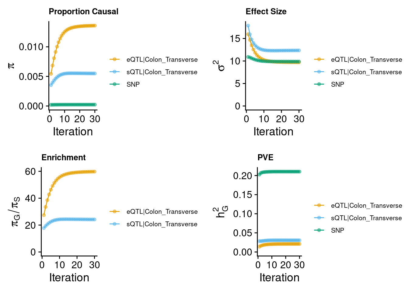
2024-09-12 13:47:19 INFO::Annotating ctwas finemapping result ...
2024-09-12 13:47:29 INFO::add gene_name and gene_type
2024-09-12 13:47:30 INFO::split PIPs for traits mapped to multiple genes
2024-09-12 13:47:30 INFO::use gene mid positions
2024-09-12 13:47:30 INFO::add SNP positions
Munro et al : 6 modalities
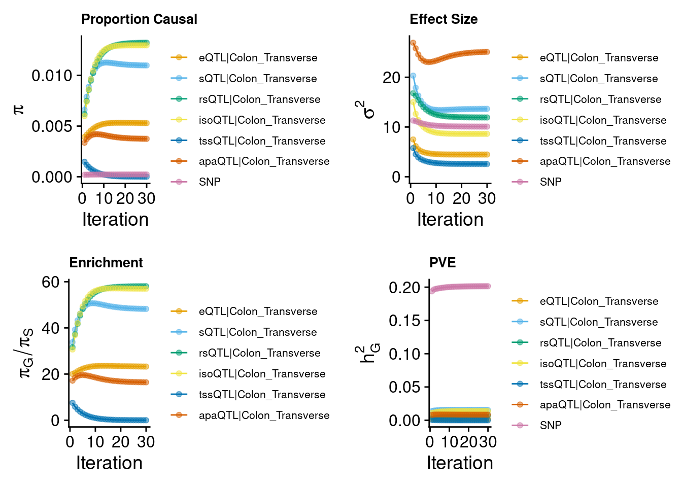
2024-09-12 13:47:55 INFO::Annotating ctwas finemapping result ...
2024-09-12 13:48:00 INFO::add gene_name and gene_type
2024-09-12 13:48:00 INFO::use gene mid positions
2024-09-12 13:48:00 INFO::add SNP positions
Compare the results from Predictdb & Munro weights
If we filter by combined pip >0.8 in both settings, we have
There’s no overlapped genes at combined_pip > 0.8.
We noticed that, when using Munro’s weights, we have GNA12 as the top1 IBD risk gene, which has been reported by literature. https://www.ncbi.nlm.nih.gov/pmc/articles/PMC10323775/
But when using predictdb weights, we missed this gene.
[1] "Locus plot -- Predictdb"2024-09-12 13:48:07 INFO::focal gene: GNA12
2024-09-12 13:48:07 INFO::focal id: ENSG00000146535.13|expression_Colon_Transverse
2024-09-12 13:48:07 INFO::plot locus range: chr7 2732556,4533638
2024-09-12 13:48:07 INFO::GNA12 Colon_Transverse eQTL QTLs
2024-09-12 13:48:07 INFO::QTL positions: 2760492,2820213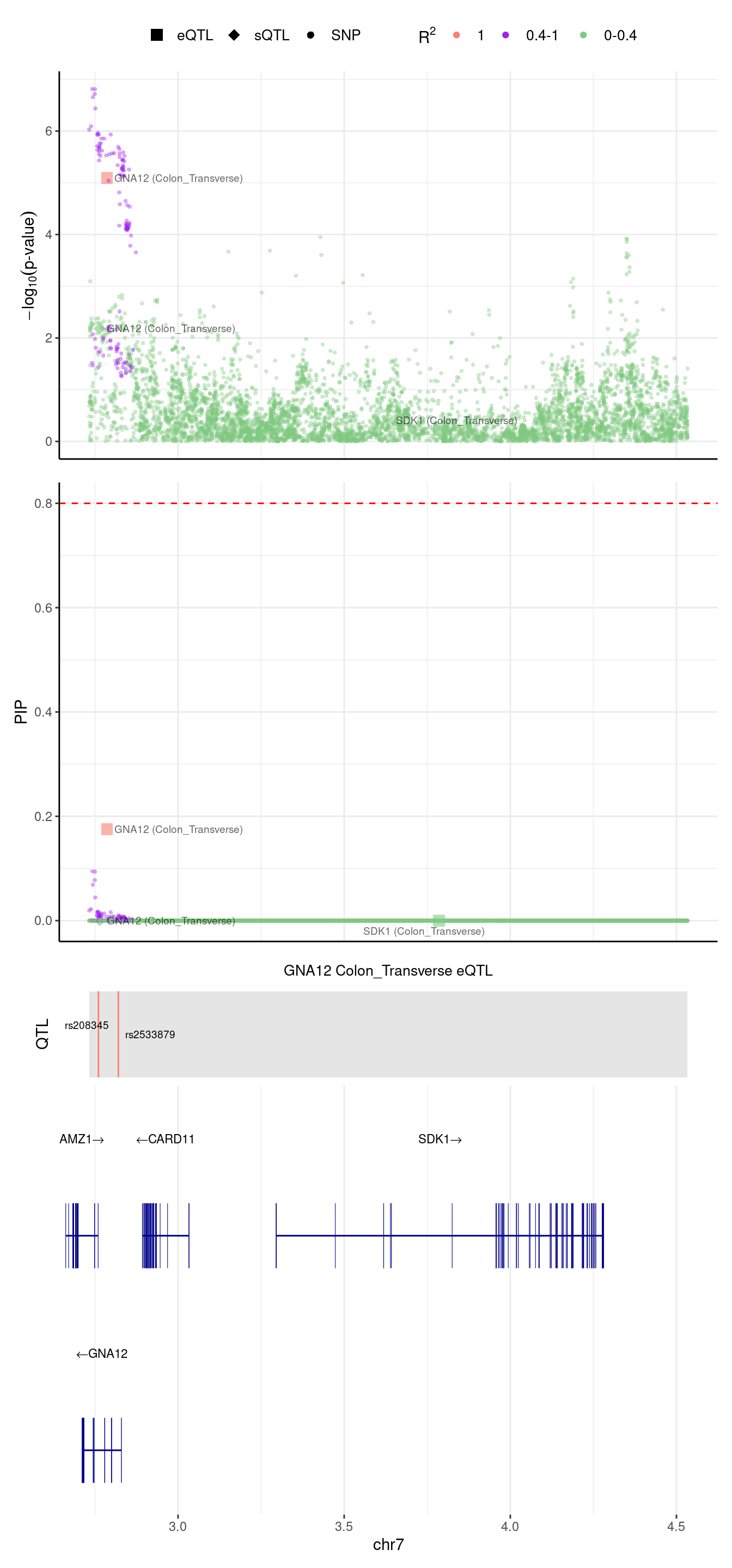
| Version | Author | Date |
|---|---|---|
| 525859b | XSun | 2024-09-10 |
[1] "Locus plot -- Munro"2024-09-12 13:48:14 INFO::focal gene: GNA12
2024-09-12 13:48:14 INFO::focal id: ENSG00000146535|expression_Colon_Transverse
2024-09-12 13:48:14 INFO::plot locus range: chr7 2732556,4533638
2024-09-12 13:48:14 INFO::GNA12 Colon_Transverse eQTL QTLs
2024-09-12 13:48:14 INFO::QTL positions: 2750246,2760492,3092158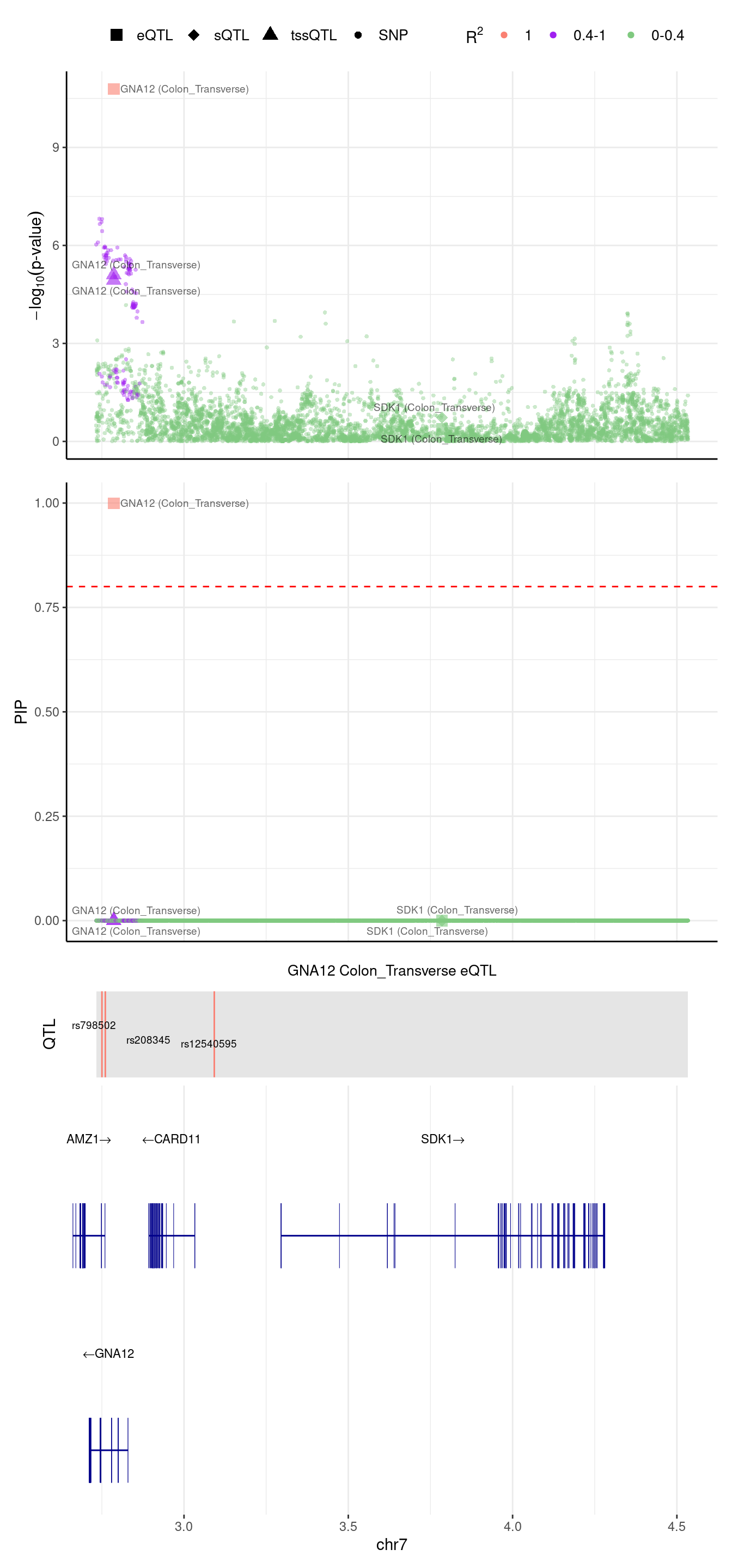
We are trying to figure out why GNA12 was missed by predictdb weights.
In predictdb eQTL model, there are 2 SNPs,
              weight
rs208345   0.0925621
rs2533879 -0.1090777
In Munro eQTL model, there are 5 SNPs,
                weight
rs755179    0.01220240
rs798544   -0.04916490
rs798502   -0.06499180
rs208345    0.03188710
rs12540595 -0.00183916
We extracted the EUR LD R2 from 1000G using https://ldlink.nih.gov/?tab=ldmatrix
We noticed that, the 2 SNPs in predictdb weights are either in Munro weights (rs208345) or in LD with the Munro eQTLs (rs2533879).
| rs755179 | rs798544 | rs798502 | rs208345 | rs12540595 | |
|---|---|---|---|---|---|
| rs208345 | 0.004 | 0.049 | 0.051 | 1.0 | 0.001 |
| rs2533879 | 0.002 | 0.8 | 0.929 | 0.051 | 0.004 |
We also noticed that, 2 (rs798502,rs798544) of the 5 Munro eQTLs are in LD with each other
| rs755179 | rs798544 | rs798502 | rs208345 | rs12540595 | |
|---|---|---|---|---|---|
| rs755179 | 1.0 | 0.003 | 0.003 | 0.004 | 0.0 |
| rs798544 | 0.003 | 1.0 | 0.838 | 0.049 | 0.005 |
| rs798502 | 0.003 | 0.838 | 1.0 | 0.051 | 0.005 |
| rs208345 | 0.004 | 0.049 | 0.051 | 1.0 | 0.001 |
| rs12540595 | 0.0 | 0.005 | 0.005 | 0.001 | 1.0 |
We checked the z scores for these SNPs,
                id A1 A2          z
4216443   rs755179  T  C  0.4172662
4217471   rs798544  C  T  4.7883212
4217631   rs798502  A  C  5.2463768
4217679   rs208345  A  G -2.0923913
4218004  rs2533879  G  A  4.7518248
4219465 rs12540595  G  A -1.7364341
The z-scores for GNA12 are:
predictdb: -4.461474
Munro: -6.736242
Checking why Predicdb results missed many Munro genes
[1] "# of Unique munro genes = 18"[1] "# of Unique munro genes included in predictdb data = 12"There are some genes have large abs(z) but low PIPs in predictdb setting (RTEL1, USP4), we make locus plots for these genes to understand why
RTEL1: this gene was assigned to region 20_63558827_64333810 in predictdb setting but 20_62670503_63558827 in Munro setting
[1] "Locus plot -- Predictdb"2024-09-12 13:48:24 INFO::focal gene: RTEL1
2024-09-12 13:48:24 INFO::focal id: intron_20_63689132_63689502|splicing_Colon_Transverse
2024-09-12 13:48:24 INFO::plot locus range: chr20 63558727,64328976
2024-09-12 13:48:24 INFO::RTEL1 Colon_Transverse sQTL QTLs
2024-09-12 13:48:24 INFO::QTL positions: 63688845,63689615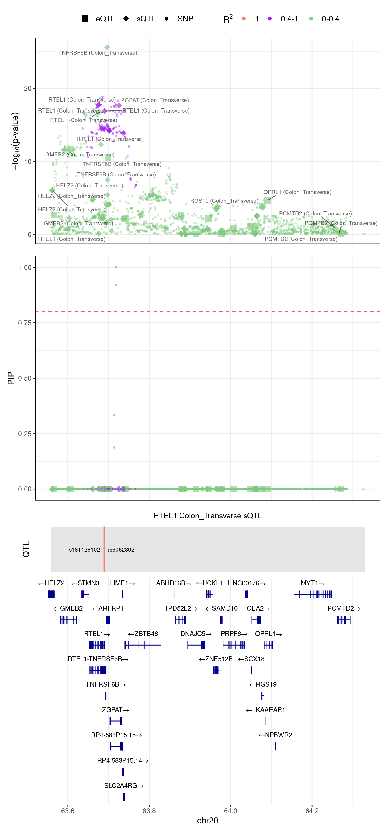
| Version | Author | Date |
|---|---|---|
| 525859b | XSun | 2024-09-10 |
We noticed in the top panel, there is a gene with outstanding pvalue, but 2 SNPs have the largest PIPs (second panel). We try to understand this case, we run ctwas in this region with L=1
[1] "the pre-estimated L for this region is 3"2024-09-12 13:48:28 INFO::Fine-mapping 1 regions ...2024-09-12 13:48:30 INFO::Annotating ctwas finemapping result ...
2024-09-12 13:48:33 INFO::add gene_name and gene_type
2024-09-12 13:48:33 INFO::split PIPs for traits mapped to multiple genes
2024-09-12 13:48:33 INFO::use gene mid positions
2024-09-12 13:48:33 INFO::add SNP positions2024-09-12 13:48:39 INFO::focal gene: TNFRSF6B
2024-09-12 13:48:39 INFO::focal id: intron_20_63695854_63696760|splicing_Colon_Transverse
2024-09-12 13:48:39 INFO::plot locus range: chr20 63558727,64328976
2024-09-12 13:48:39 INFO::TNFRSF6B Colon_Transverse sQTL QTLs
2024-09-12 13:48:39 INFO::QTL positions: 63697746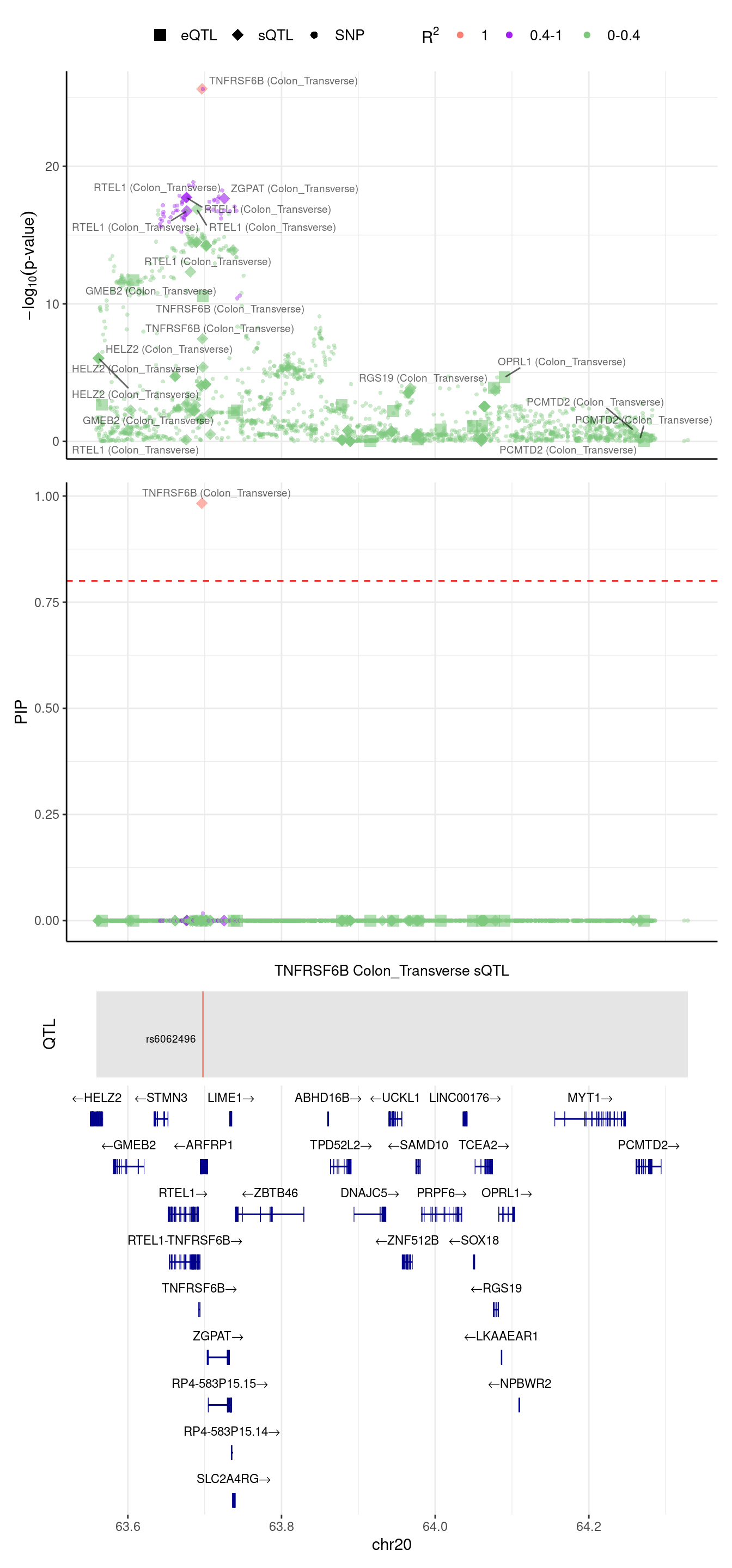
| Version | Author | Date |
|---|---|---|
| 525859b | XSun | 2024-09-10 |
[1] "Locus plot -- Munro"2024-09-12 13:48:42 INFO::focal gene: RTEL1
2024-09-12 13:48:42 INFO::focal id: ENSG00000258366:ENST00000370003|isoform_Colon_Transverse
2024-09-12 13:48:42 INFO::plot locus range: chr20 62664015,63677132
2024-09-12 13:48:43 INFO::RTEL1 Colon_Transverse isoQTL QTLs
2024-09-12 13:48:43 INFO::QTL positions: 63403750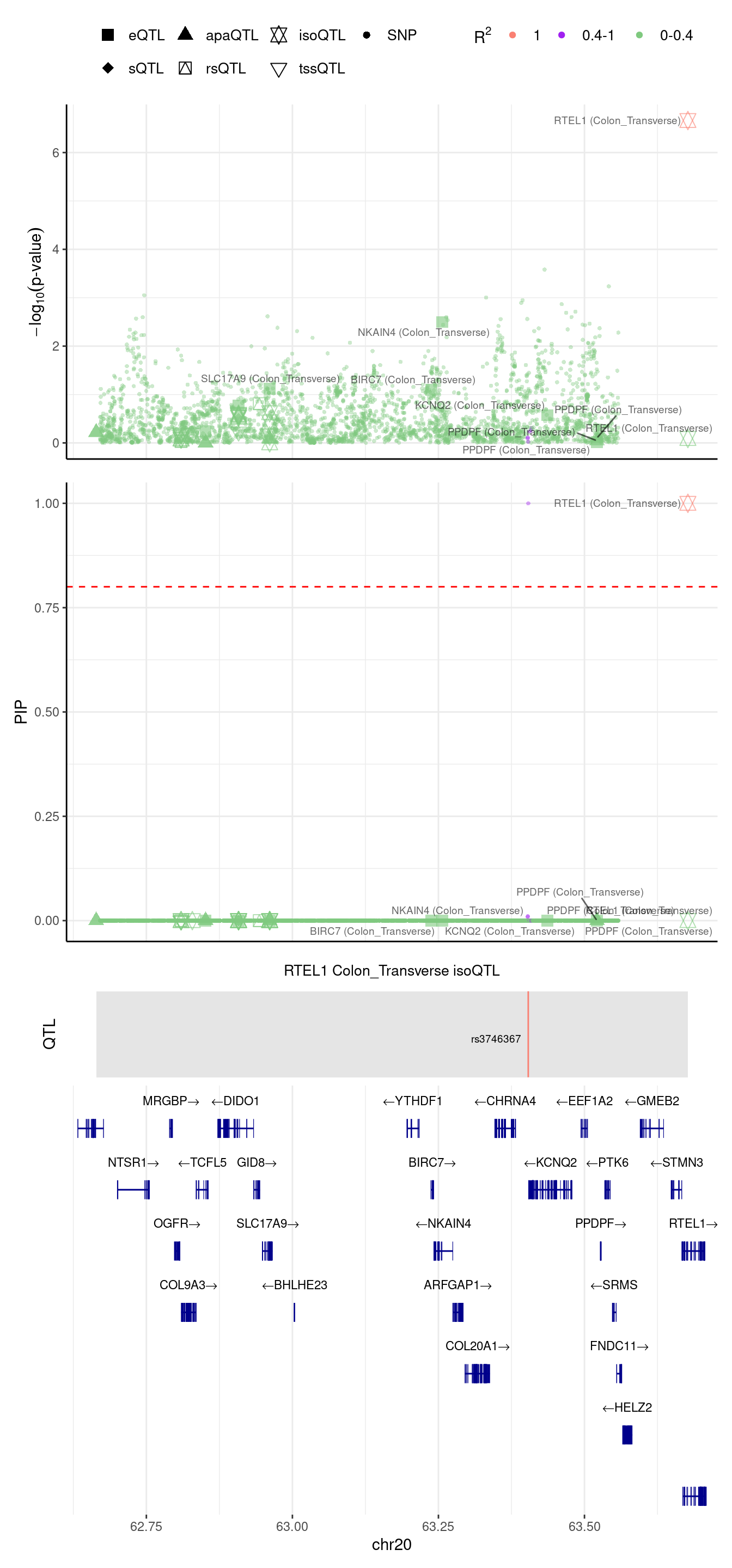
| Version | Author | Date |
|---|---|---|
| 525859b | XSun | 2024-09-10 |
If we merge the RTEL1 region
2024-09-12 13:48:46 INFO::focal gene: RTEL1
2024-09-12 13:48:46 INFO::focal id: ENSG00000258366:ENST00000370003|isoform_Colon_Transverse
2024-09-12 13:48:46 INFO::plot locus range: chr20 62664015,64328976
2024-09-12 13:48:47 INFO::RTEL1 Colon_Transverse isoQTL QTLs
2024-09-12 13:48:47 INFO::QTL positions: 63403750,63701763,63785828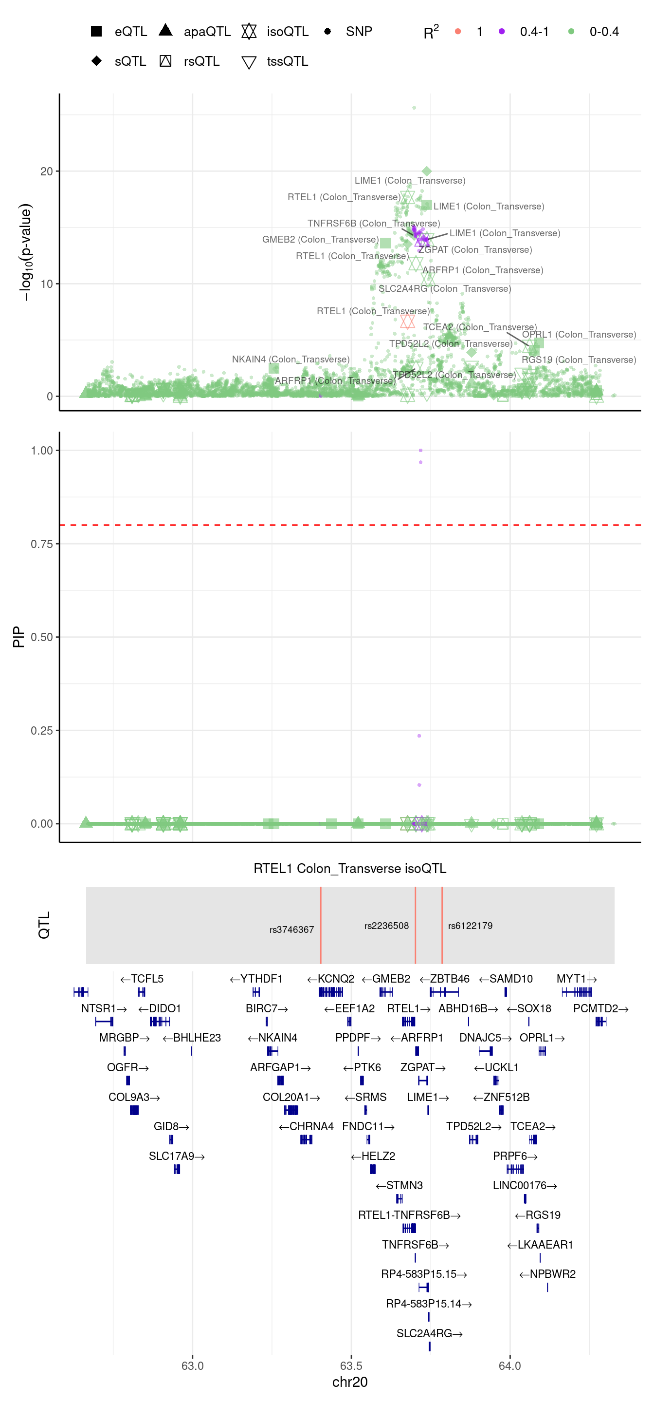
| Version | Author | Date |
|---|---|---|
| 525859b | XSun | 2024-09-10 |
USP4: this gene was assigned to region 3_49279539_51797999 in predictdb setting but 3_47685722_49279539 in Munro setting
[1] "Locus plot -- Predictdb"2024-09-12 13:48:51 INFO::focal gene: LAMB2
2024-09-12 13:48:51 INFO::focal id: intron_3_49125169_49125269|splicing_Colon_Transverse
2024-09-12 13:48:51 INFO::plot locus range: chr3 47688075,49277627
2024-09-12 13:48:52 INFO::LAMB2 Colon_Transverse sQTL QTLs
2024-09-12 13:48:52 INFO::QTL positions: 49124851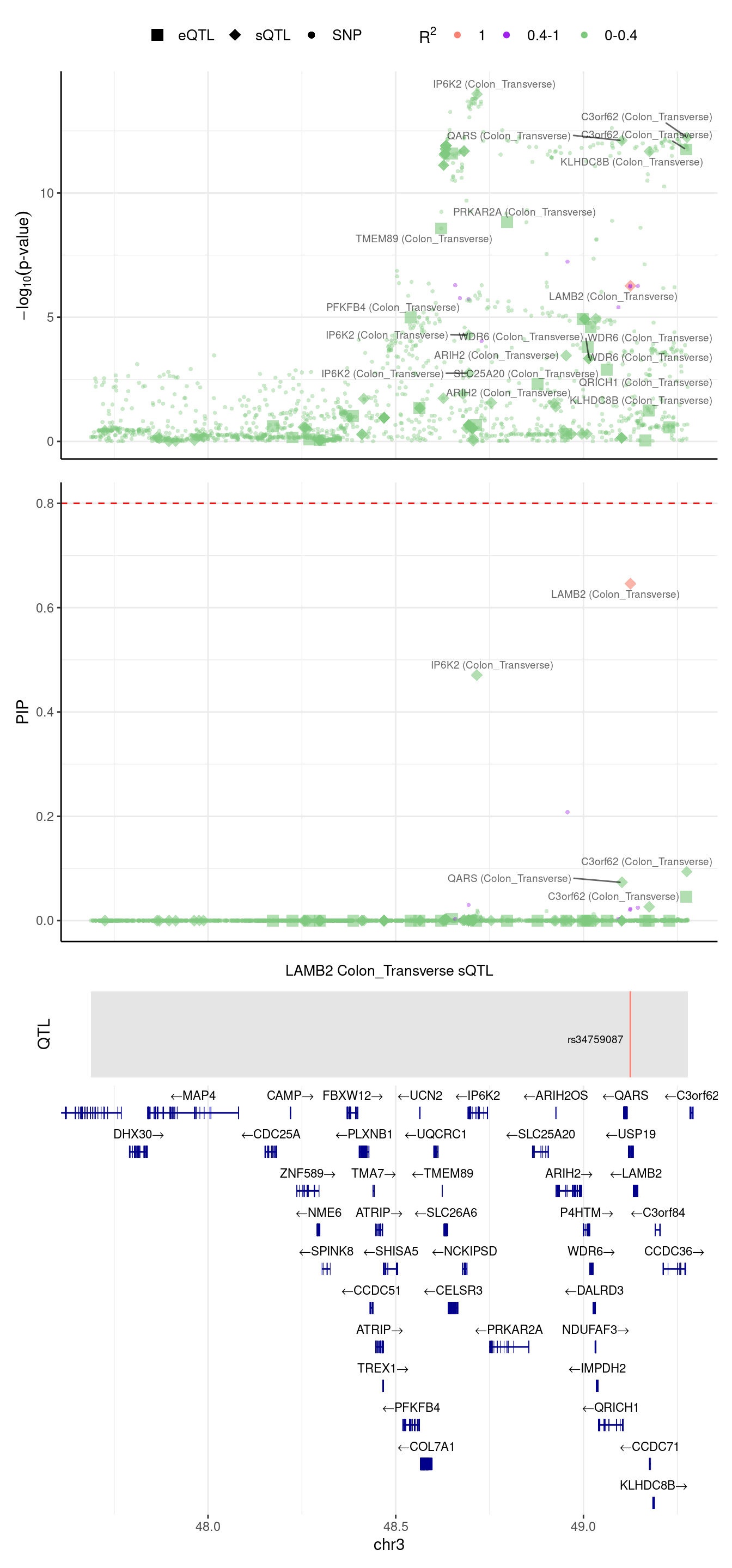
2024-09-12 13:48:54 INFO::focal gene: USP4
2024-09-12 13:48:54 INFO::focal id: ENSG00000114316.12|expression_Colon_Transverse
2024-09-12 13:48:54 INFO::plot locus range: chr3 49279498,51794719
2024-09-12 13:48:55 INFO::USP4 Colon_Transverse eQTL QTLs
2024-09-12 13:48:55 INFO::QTL positions: 49340655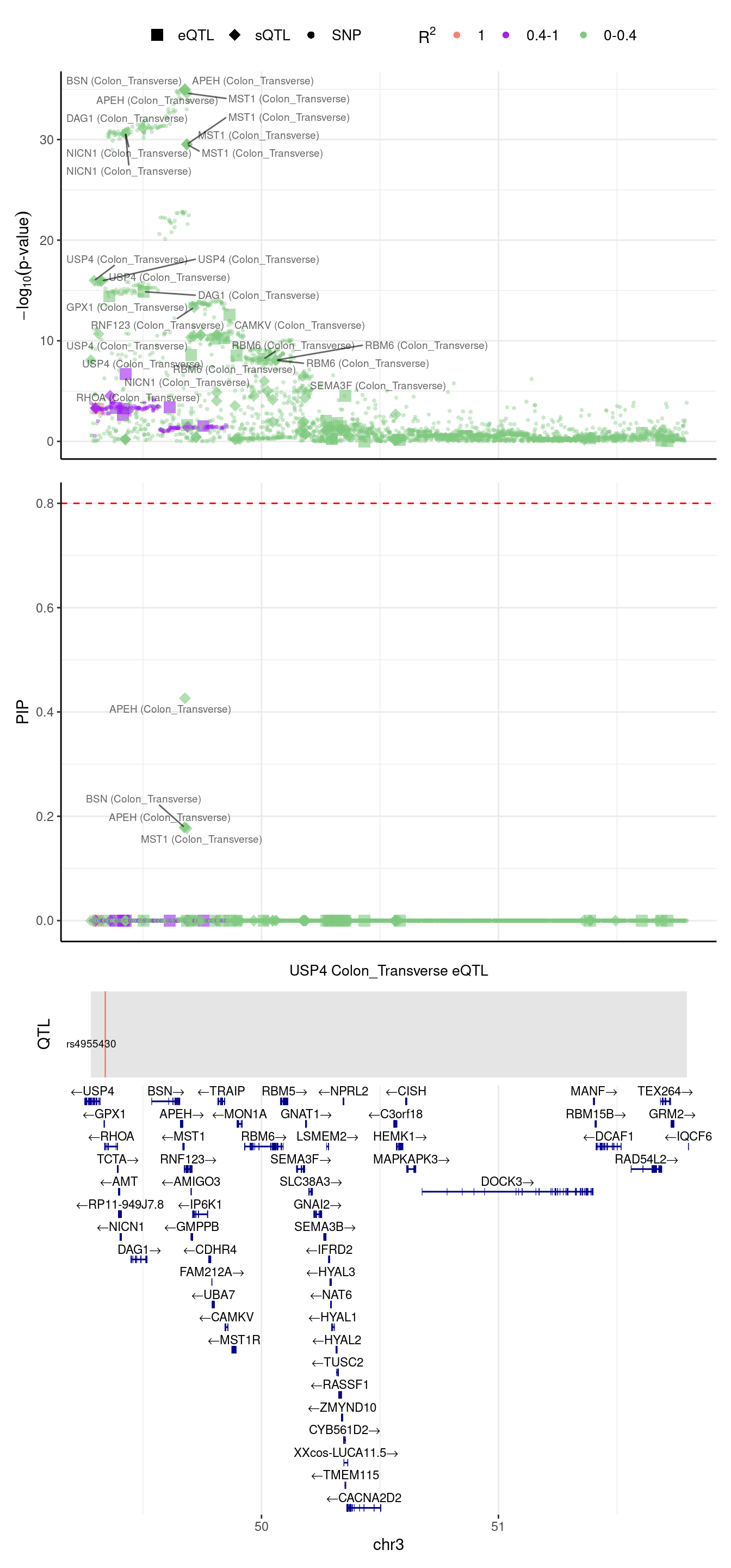
[1] "Locus plot -- Munro"2024-09-12 13:49:02 INFO::focal gene: USP4
2024-09-12 13:49:02 INFO::focal id: ENSG00000114316.grp_1.downstream.ENST00000265560|apa_Colon_Transverse
2024-09-12 13:49:02 INFO::plot locus range: chr3 47255638,49426236
2024-09-12 13:49:02 INFO::USP4 Colon_Transverse apaQTL QTLs
2024-09-12 13:49:02 INFO::QTL positions: 48845667,48945299,49141557,49178533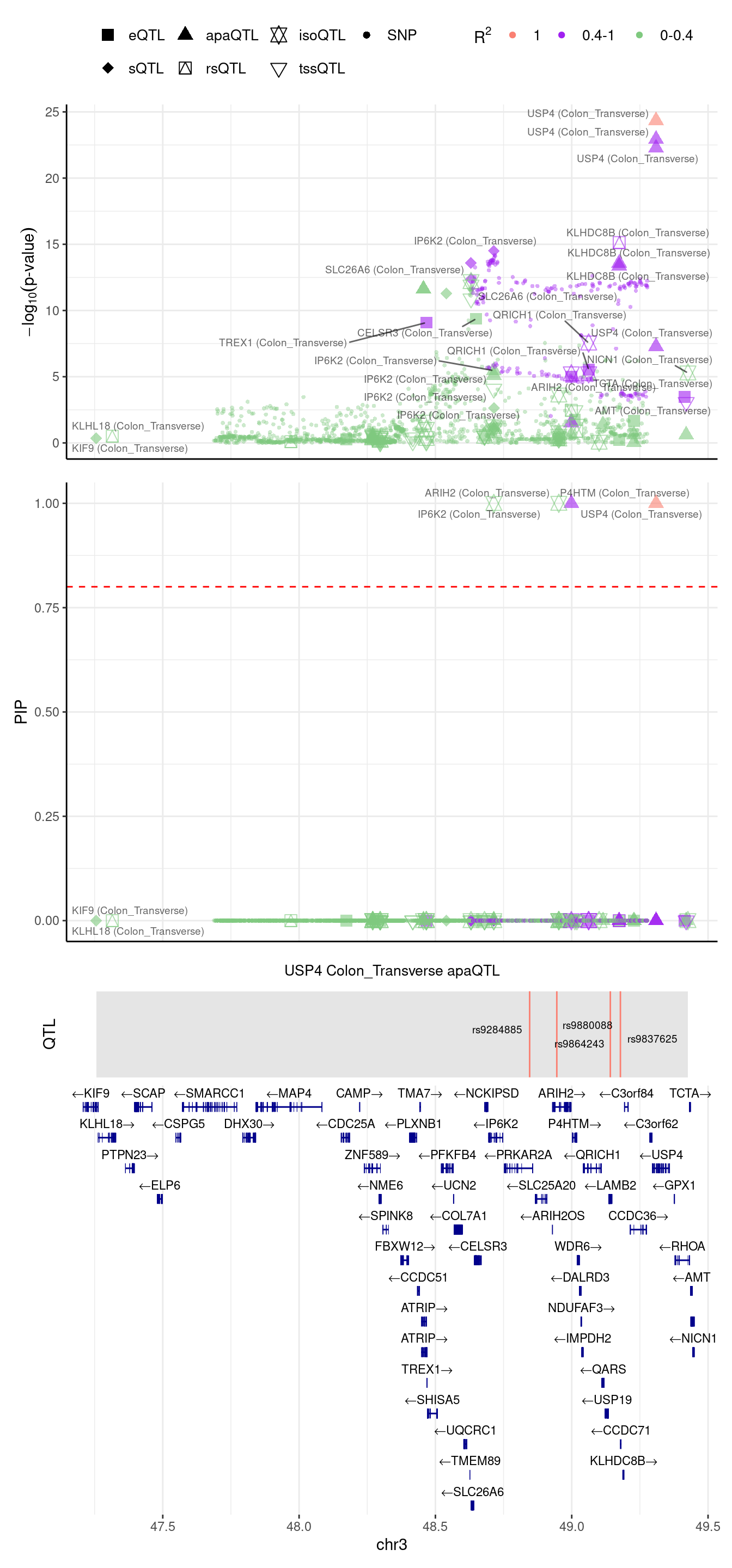
2024-09-12 13:49:05 INFO::focal gene: MST1
2024-09-12 13:49:05 INFO::focal id: ENSG00000173531:chr3:49684189:49684314:clu_47947_-|splicing_Colon_Transverse
2024-09-12 13:49:05 INFO::plot locus range: chr3 48998420,51794719
2024-09-12 13:49:05 INFO::MST1 Colon_Transverse sQTL QTLs
2024-09-12 13:49:05 INFO::QTL positions: 49298312,49322510,49345492,49603616,49641218,49644878,49665051,49674864,49682296,49694428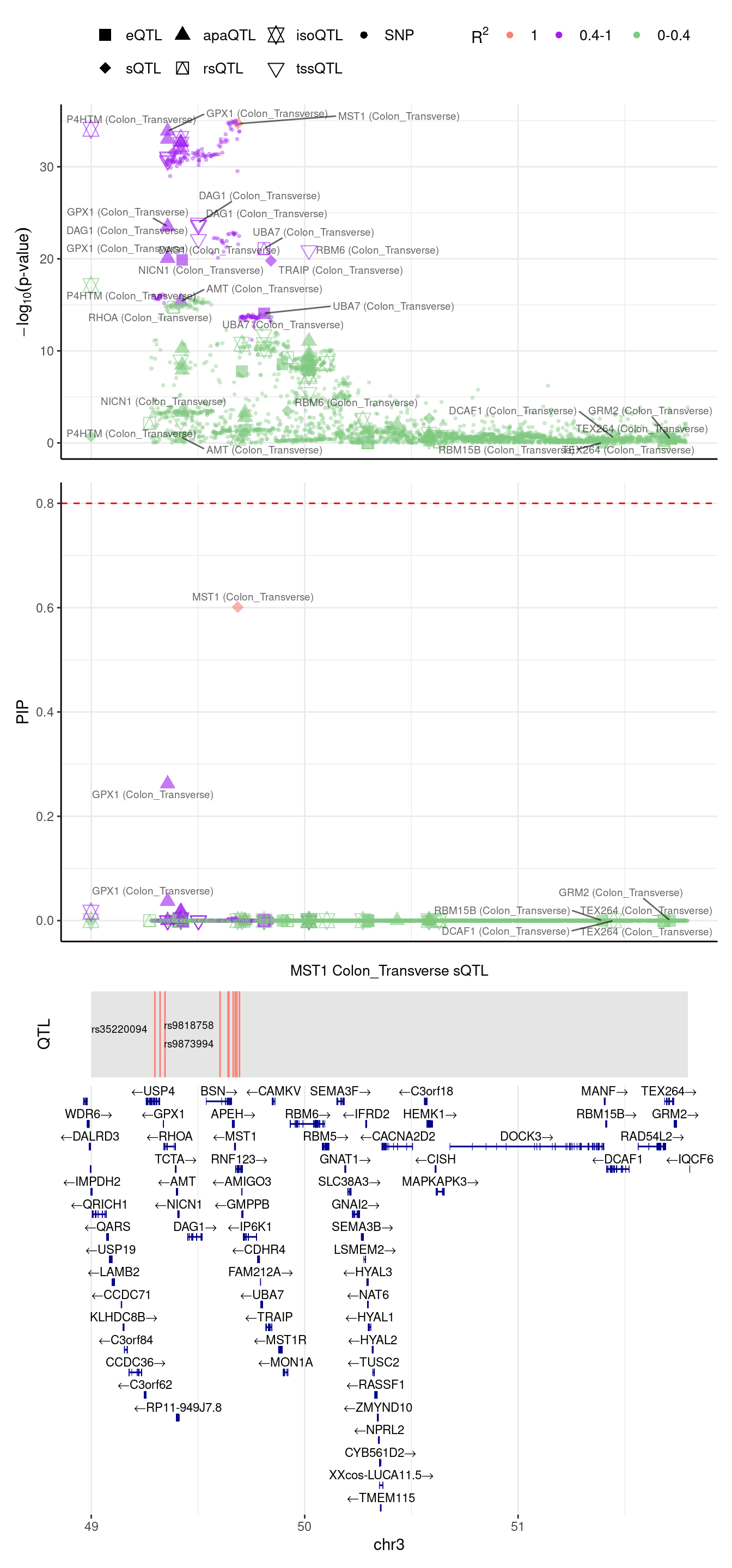
| Version | Author | Date |
|---|---|---|
| 525859b | XSun | 2024-09-10 |
If we merge the 2 regions above
2024-09-12 13:49:12 INFO::focal gene: USP4
2024-09-12 13:49:12 INFO::focal id: ENSG00000114316.grp_2.downstream.ENST00000265560|apa_Colon_Transverse
2024-09-12 13:49:12 INFO::plot locus range: chr3 47255638,51794719
2024-09-12 13:49:13 INFO::USP4 Colon_Transverse apaQTL QTLs
2024-09-12 13:49:13 INFO::QTL positions: 48845667,48945299,49124851,49178533,49288745,49306168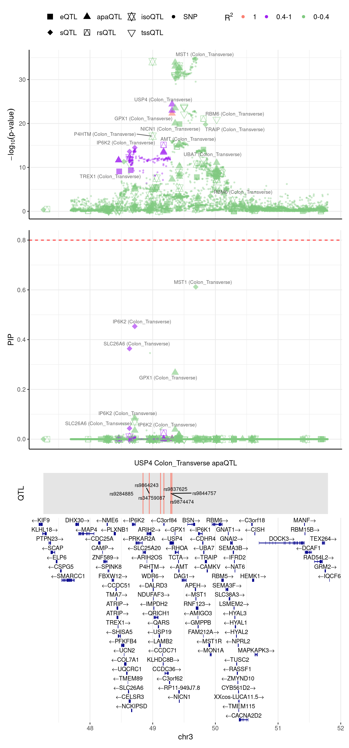
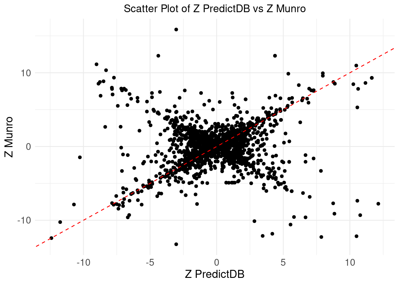
Comparing z-scores
library(dplyr)

gene_predictdb <- finemap_res_predictdb[finemap_res_predictdb$type !="SNP",]
gene_predictdb <- gene_predictdb[,c("gene_name","z","susie_pip")]

gene_predictdb_clean <- gene_predictdb %>%
  group_by(gene_name) %>%
  dplyr::filter(abs(z) == max(abs(z))) %>%
  ungroup()

gene_munro <- finemap_res_munro[finemap_res_munro$type !="SNP",]
gene_munro <- gene_munro[,c("gene_name","z","susie_pip")]

gene_munro_clean <- gene_munro %>%
  group_by(gene_name) %>%
  dplyr::filter(abs(z) == max(abs(z))) %>%
  ungroup()

merge_eqtl <- merge(gene_predictdb_clean, gene_munro_clean, by="gene_name")
colnames(merge_eqtl) <- c("gene_name","z_predictdb", "pip_predictdb","z_munro", "pip_munro")


ggplot(merge_eqtl, aes(x = z_predictdb, y = z_munro)) +
  geom_point() +
  geom_abline(intercept = 0, slope = 1, color = "red", linetype = "dashed") +  # Add y=x line
  theme_minimal() +
  labs(
    x = "Z PredictDB",
    y = "Z Munro",
    title = "Scatter Plot of Z PredictDB vs Z Munro"
  ) +
   theme(
    plot.title = element_text(hjust = 0.5),
    axis.text = element_text(size = 12),
    axis.title = element_text(size = 14),
    legend.position = "none"  # Remove the legend
  )
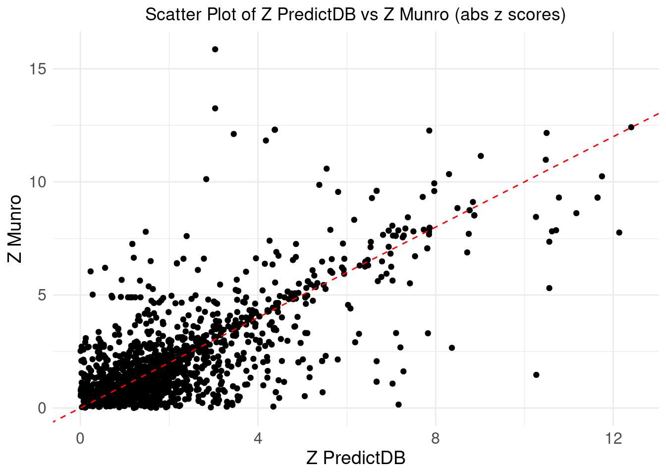
print("we take the abs(z)")[1] "we take the abs(z)"merge_eqtl$z_predictdb <- abs(merge_eqtl$z_predictdb)
merge_eqtl$z_munro <- abs(merge_eqtl$z_munro)
ggplot(merge_eqtl, aes(x = z_predictdb, y = z_munro)) +
geom_point() +
geom_abline(intercept = 0, slope = 1, color = "red", linetype = "dashed") + # Add y=x line
theme_minimal() +
labs(
x = "Z PredictDB",
y = "Z Munro",
title = "Scatter Plot of Z PredictDB vs Z Munro (abs z scores)"
) +
theme(
plot.title = element_text(hjust = 0.5),
axis.text = element_text(size = 12),
axis.title = element_text(size = 14),
legend.position = "none" # Remove the legend
)
gene_predictdb <- finemap_res_predictdb[finemap_res_predictdb$type =="eQTL",]
gene_predictdb <- gene_predictdb[,c("gene_name","z","susie_pip")]
gene_munro <- finemap_res_munro[finemap_res_munro$type =="eQTL",]
gene_munro <- gene_munro[,c("gene_name","z","susie_pip")]

merge_eqtl <- merge(gene_predictdb, gene_munro, by="gene_name")
colnames(merge_eqtl) <- c("gene_name","z_predictdb", "pip_predictdb","z_munro", "pip_munro")

merge_eqtl <- data.frame(lapply(merge_eqtl, function(x) {
  if(is.numeric(x)) format(round(x, 4), nsmall = 4)
  else x
}))


merge_eqtl$label <- ifelse(merge_eqtl$gene_name %in% overlapped_gene_all$genename, merge_eqtl$gene_name, NA)

merge_eqtl$z_predictdb <- as.numeric(merge_eqtl$z_predictdb)
merge_eqtl$z_munro<- as.numeric(merge_eqtl$z_munro)
merge_eqtl$pip_predictdb <- as.numeric(merge_eqtl$pip_predictdb)
merge_eqtl$pip_munro<- as.numeric(merge_eqtl$pip_munro)

# Create the scatter plot with labels for specific genes
ggplot(merge_eqtl, aes(x = z_predictdb, y = z_munro)) +
  geom_point(aes(color = !is.na(label))) +  # Color based on whether label is NA
  geom_abline(intercept = 0, slope = 1, color = "red", linetype = "dashed") +  # Add y=x line
  theme_minimal() +
  labs(
    x = "Z PredictDB",
    y = "Z Munro",
    title = "Scatter Plot of Z PredictDB vs Z Munro"
  ) +
  geom_text(aes(label = label), vjust = 1.5, hjust = 1.5, size = 3, color = "red") +  # Label the points with red color
  scale_color_manual(values = c("black", "red")) +  # Set colors: black for non-labeled, red for labeled
  theme(
    plot.title = element_text(hjust = 0.5),
    axis.text = element_text(size = 12),
    axis.title = element_text(size = 14),
    legend.position = "none"  # Remove the legend
  )
Warning: Removed 563 rows containing missing values or values outside the scale range
(`geom_text()`).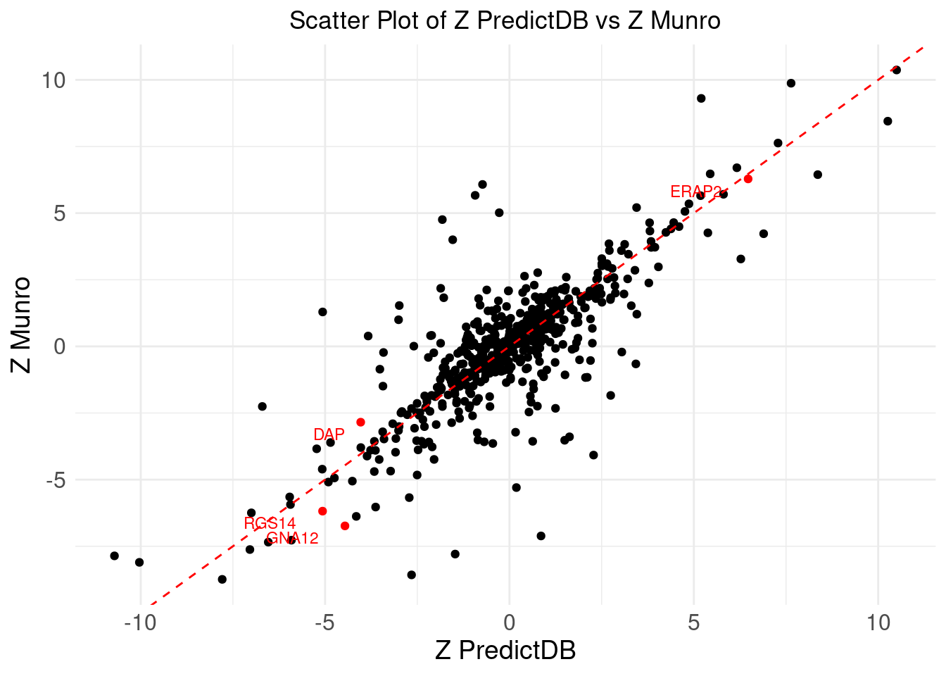
ggplot(merge_eqtl, aes(x = pip_predictdb, y = pip_munro)) +
  geom_point(aes(color = !is.na(label))) +  # Color based on whether label is NA
  geom_abline(intercept = 0, slope = 1, color = "red", linetype = "dashed") +  # Add y=x line
  theme_minimal() +
  labs(
    x = "PIP PredictDB",
    y = "PIP Munro",
    title = "Scatter Plot of PIP PredictDB vs PIP Munro"
  ) +
  geom_text(aes(label = label), vjust = 1.5, hjust = 1.5, size = 3, color = "red") +  # Label the points with red color
  scale_color_manual(values = c("black", "red")) +  # Set colors: black for non-labeled, red for labeled
  theme(
    plot.title = element_text(hjust = 0.5),
    axis.text = element_text(size = 12),
    axis.title = element_text(size = 14),
    legend.position = "none"  # Remove the legend
  )
Warning: Removed 563 rows containing missing values or values outside the scale range
(`geom_text()`).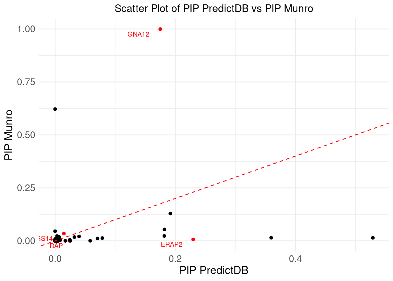
DT::datatable(merge_eqtl,caption = htmltools::tags$caption( style = 'caption-side: topleft; text-align = left; color:black;','Z-scores and PIPs computed from eQTL, for the overlapped genes'),options = list(pageLength = 5) )If we don’t consider CS, I noticed there is a gene NXPE1. The z-predictdb = 4.5985 and z-munro = 4.4947. But pip_predictdb = 0.5289 and pip_munro = 0.0142.
In predictdb eQTL model, there are 1 SNPs,
             weight
rs661946 0.07486575
In Munro eQTL model, there are 3 SNPs,
               weight
rs238925  -0.00283751
rs561722   0.27416500
rs1850521 -0.02065090
We checked the z scores for these SNPs,
               id A1 A2         z
6612785  rs238925  G  T 1.8692308
6614255  rs561722  C  T 4.6439394
6614384  rs661946  C  T 4.5984848
6614420 rs1850521  G  T 0.3854749
The both predictdb eQTL and munro eQTLs have large GWAS z-score. We checked more about the finemapping results
The Munro PIPs are from sQTLs. So, as shown in the earlier scatter plot, the eQTL PIP is very low.
sessionInfo()R version 4.2.0 (2022-04-22)
Platform: x86_64-pc-linux-gnu (64-bit)
Running under: CentOS Linux 7 (Core)
Matrix products: default
BLAS/LAPACK: /software/openblas-0.3.13-el7-x86_64/lib/libopenblas_haswellp-r0.3.13.so
locale:
[1] C
attached base packages:
[1] stats4 stats graphics grDevices utils datasets methods
[8] base
other attached packages:
[1] cowplot_1.1.1 ggrepel_0.9.1
[3] locuszoomr_0.2.1 logging_0.10-108
[5] EnsDb.Hsapiens.v86_2.99.0 ensembldb_2.20.2
[7] AnnotationFilter_1.20.0 GenomicFeatures_1.48.3
[9] AnnotationDbi_1.58.0 Biobase_2.56.0
[11] GenomicRanges_1.48.0 GenomeInfoDb_1.39.9
[13] IRanges_2.30.0 S4Vectors_0.34.0
[15] BiocGenerics_0.42.0 gridExtra_2.3
[17] forcats_0.5.1 stringr_1.5.1
[19] dplyr_1.1.4 purrr_1.0.2
[21] readr_2.1.2 tidyr_1.3.0
[23] tibble_3.2.1 ggplot2_3.5.1
[25] tidyverse_1.3.1 data.table_1.14.2
[27] ctwas_0.4.11
loaded via a namespace (and not attached):
[1] readxl_1.4.0 backports_1.4.1
[3] workflowr_1.7.0 BiocFileCache_2.4.0
[5] lazyeval_0.2.2 BiocParallel_1.30.3
[7] crosstalk_1.2.0 LDlinkR_1.2.3
[9] digest_0.6.29 htmltools_0.5.2
[11] fansi_1.0.3 magrittr_2.0.3
[13] memoise_2.0.1 tzdb_0.4.0
[15] Biostrings_2.64.0 modelr_0.1.8
[17] matrixStats_0.62.0 prettyunits_1.1.1
[19] colorspace_2.0-3 blob_1.2.3
[21] rvest_1.0.2 rappdirs_0.3.3
[23] haven_2.5.0 xfun_0.41
[25] crayon_1.5.1 RCurl_1.98-1.7
[27] jsonlite_1.8.0 zoo_1.8-10
[29] glue_1.6.2 gtable_0.3.0
[31] zlibbioc_1.42.0 XVector_0.36.0
[33] DelayedArray_0.22.0 RcppZiggurat_0.1.6
[35] scales_1.3.0 DBI_1.2.2
[37] Rcpp_1.0.12 viridisLite_0.4.0
[39] progress_1.2.2 bit_4.0.4
[41] DT_0.22 htmlwidgets_1.5.4
[43] httr_1.4.3 ellipsis_0.3.2
[45] pkgconfig_2.0.3 XML_3.99-0.14
[47] farver_2.1.0 sass_0.4.1
[49] dbplyr_2.1.1 utf8_1.2.2
[51] tidyselect_1.2.0 labeling_0.4.2
[53] rlang_1.1.2 later_1.3.0
[55] munsell_0.5.0 pgenlibr_0.3.3
[57] cellranger_1.1.0 tools_4.2.0
[59] cachem_1.0.6 cli_3.6.1
[61] generics_0.1.2 RSQLite_2.3.1
[63] broom_0.8.0 evaluate_0.15
[65] fastmap_1.1.0 yaml_2.3.5
[67] knitr_1.39 bit64_4.0.5
[69] fs_1.5.2 KEGGREST_1.36.3
[71] whisker_0.4 xml2_1.3.3
[73] biomaRt_2.54.1 compiler_4.2.0
[75] rstudioapi_0.13 plotly_4.10.0
[77] filelock_1.0.2 curl_4.3.2
[79] png_0.1-7 reprex_2.0.1
[81] bslib_0.3.1 stringi_1.7.6
[83] highr_0.9 lattice_0.20-45
[85] ProtGenerics_1.28.0 Matrix_1.5-3
[87] vctrs_0.6.5 pillar_1.9.0
[89] lifecycle_1.0.4 jquerylib_0.1.4
[91] bitops_1.0-7 irlba_2.3.5
[93] httpuv_1.6.5 rtracklayer_1.56.0
[95] R6_2.5.1 BiocIO_1.6.0
[97] promises_1.2.0.1 codetools_0.2-18
[99] assertthat_0.2.1 SummarizedExperiment_1.26.1
[101] rprojroot_2.0.3 rjson_0.2.21
[103] withr_2.5.0 GenomicAlignments_1.32.0
[105] Rsamtools_2.12.0 GenomeInfoDbData_1.2.8
[107] parallel_4.2.0 hms_1.1.1
[109] grid_4.2.0 gggrid_0.2-0
[111] rmarkdown_2.25 Rfast_2.0.7
[113] MatrixGenerics_1.8.0 git2r_0.30.1
[115] mixsqp_0.3-43 lubridate_1.8.0
[117] restfulr_0.0.14