Last updated: 2025-03-24

Checks: 6 1

Knit directory: multigroup_ctwas_analysis/

This reproducible R Markdown analysis was created with workflowr (version 1.7.0). The Checks tab describes the reproducibility checks that were applied when the results were created. The Past versions tab lists the development history.

R Markdown file: uncommitted changes

The R Markdown is untracked by Git. To know which version of the R Markdown file created these results, you’ll want to first commit it to the Git repo. If you’re still working on the analysis, you can ignore this warning. When you’re finished, you can run wflow_publish to commit the R Markdown file and build the HTML.

Environment: empty

Great job! The global environment was empty. Objects defined in the global environment can affect the analysis in your R Markdown file in unknown ways. For reproduciblity it’s best to always run the code in an empty environment.

Seed: set.seed(20231112)

The command set.seed(20231112) was run prior to running the code in the R Markdown file. Setting a seed ensures that any results that rely on randomness, e.g. subsampling or permutations, are reproducible.

Session information: recorded

Great job! Recording the operating system, R version, and package versions is critical for reproducibility.

Cache: none

Nice! There were no cached chunks for this analysis, so you can be confident that you successfully produced the results during this run.

File paths: relative

Great job! Using relative paths to the files within your workflowr project makes it easier to run your code on other machines.

Repository version: 7f6f7b1

Great! You are using Git for version control. Tracking code development and connecting the code version to the results is critical for reproducibility.

The results in this page were generated with repository version 7f6f7b1. See the Past versions tab to see a history of the changes made to the R Markdown and HTML files.

Note that you need to be careful to ensure that all relevant files for the analysis have been committed to Git prior to generating the results (you can use wflow_publish or wflow_git_commit). workflowr only checks the R Markdown file, but you know if there are other scripts or data files that it depends on. Below is the status of the Git repository when the results were generated:


Ignored files:
    Ignored:    .Rhistory
    Ignored:    cv/

Untracked files:
    Untracked:  analysis/data_weight_training_avg.Rmd

Note that any generated files, e.g. HTML, png, CSS, etc., are not included in this status report because it is ok for generated content to have uncommitted changes.

There are no past versions. Publish this analysis with wflow_publish() to start tracking its development.

Introduction

Data source

Normalized RNA phenotype were shared by Munro et al

Covariates are downloaded from https://pantry.pejlab.org/

Genotype are from gtex v8, we imputed the missing genotype using beagle

Workflow

Cross validation

For each RNA phenotype in each tissue, we partitioned the available samples into training (80%) and testing (20%) datasets.

Training Phase

For each RNA molecular, we performed the following steps:

Variant Selection: We defined a ±50 kb window around the transcription start site (TSS) of each gene, following Munro et al. Variants located within this window were selected for analysis.
Preprocessing: Covariates were regressed out from both the RNA phenotype and the genotype matrix containing the selected variants. The residuals from this regression were used as inputs for subsequent analysis. (as susie tutorial described)
Fine-Mapping with SuSiE: We applied SuSiE with L = 1 and L = 5 to the residualized data and identified the top variants from the credible sets.
Effect Size Estimation: For the selected variants, we re-fitted a multiple linear regression model:
```
model <- lm(scaled_RNA_phenotype ~ SNPs_centered + covariates_scaled)
effect_sizes <- coef(model)
```
where scaled_RNA_phenotype represents the scaled RNA phenotype, SNPs_centered denotes the centered SNP genotype matrix, and covariates_scaled represents scaled covariates. The estimated coefficients from this model were used as effect sizes for the selected SNPs.

Testing Phase

Using the trained effect sizes, we predicted RNA phenotypes in the testing dataset and evaluated model performance.

Evaluation

We used MSE, r2 to evaluate the performance of the prediction model

\[ R^2 = 1 - \frac{\sum (y_{\text{test}} - y_{\text{pred}})^2}{\sum (y_{\text{test}} - \bar{y}_{\text{test}})^2} \]

\(y_{\text{test}}\): Observed values in the test set,
\(y_{\text{pred}}\): Predicted values,
\(\bar{y}_{\text{test}}\): Mean of the test set observed values.

MSE

\[ \text{MSE} = \frac{1}{n} \sum_{i=1}^n (y_i - \hat{y}_i)^2 \]

\(y_i\): Observed value for the \(i\)-th sample,
\(\hat{y}_i\): Predicted value for the \(i\)-th sample,
\(n\): Total number of samples.

We performed five rounds of cross-validation and calculated the average values. Some genes had weights in certain rounds but not in others, as SuSiE did not identify credible sets. We set the threshold at 3, meaning that if a gene had an r² value from at least three rounds, we computed its mean r².”

library(RSQLite)
library(ggplot2)
library(gridExtra)

name_mapping <- read.table("/project2/xinhe/shared_data/multigroup_ctwas/weights/files_Munro/Munro_name_mapping.txt")
colnames(name_mapping) <- c("Munro_name","gtex_name")

Comparing L=1 and L=5

RNA stability

qtl = "stability"

L=1
folder_pred_L1 <- paste0("/project/xinhe/xsun/weights_training/cv/multiplesets/",qtl,"/L",L,"/rsq_summary/")
folder_sample_L1<- paste0("/project/xinhe/xsun/weights_training/cv/samples/",qtl,"/")

L=5
folder_pred_L5 <- paste0("/project/xinhe/xsun/weights_training/cv/multiplesets/",qtl,"/L",L,"/rsq_summary/")
folder_sample_L5<- paste0("/project/xinhe/xsun/weights_training/cv/samples/",qtl,"/")
folder_round1 <- paste0("/project/xinhe/xsun/weights_training/cv/multiplesets/",qtl,"/L",L,"/round1/")

sum <- c()
p <- list()
for (tissue in name_mapping$Munro_name) {
  
  if(!file.exists(paste0(folder_pred_L1,tissue,"_rsq_fusion.RDS")) | !file.exists(paste0(folder_pred_L5,tissue,"_rsq_fusion.RDS"))) next
  
  tissue_gtex <- name_mapping$gtex_name[which(name_mapping$Munro_name == tissue)]
  
  ## sample size 
  sample_test <- readRDS(paste0(folder_round1,tissue,"_samples_testing.RDS"))
  sample_test <- length(sample_test)
  sample_train <- readRDS(paste0(folder_round1,tissue,"_samples_training.RDS"))
  sample_train <- length(sample_train)
  sample_total <- sample_test + sample_train 
  
  ## L=1
  rsq_L1 <- readRDS(paste0(folder_pred_L1, tissue, "_rsq_fusion.RDS"))
  n_withcs_L1 <- nrow(rsq_L1)
  n_posrsq_L1 <- sum(rsq_L1$mean_rsq>0,na.rm = T)
  
  ## L=5
  rsq_L5 <- readRDS(paste0(folder_pred_L5, tissue, "_rsq_fusion.RDS"))
  n_withcs_L5 <- nrow(rsq_L5)
  n_posrsq_L5 <- sum(rsq_L5$mean_rsq>0,na.rm = T)
  
  n_overlap_withcs <- sum(rsq_L1$gene %in% rsq_L5$gene)
  n_overlap_posrsq <- sum(rsq_L1$gene[rsq_L1$mean_rsq > 0] %in% rsq_L1$gene[rsq_L5$mean_rsq > 0])
  
  ## total rna & average qtl
  weights <- readRDS(paste0(folder_round1, tissue, "_training_effectsizes.RDS"))
  n_rna <- length(weights)
  
  weights_nonnull <- Filter(Negate(is.null), weights)
  avg_qtl <- mean(unlist(lapply(weights_nonnull,length)),na.rm = T)
  
  tmp_tissue <- c(tissue_gtex,sample_total, n_rna, n_withcs_L1, n_withcs_L5,round(avg_qtl,digits = 4), n_overlap_withcs, n_posrsq_L1, n_posrsq_L5, n_overlap_posrsq)
  sum <- rbind(sum, tmp_tissue)
  
  rsq_L1_df <- data.frame(id = rsq_L1$gene, rsq_L1 = rsq_L1$mean_rsq)
  rsq_L5_df <- data.frame(id = rsq_L5$gene, rsq_L5 = rsq_L5$mean_rsq)
  
  rsq_merge <- merge(rsq_L1_df, rsq_L5_df , by = "id")
  
  p[[tissue_gtex]] <-  ggplot(rsq_merge, aes(x=rsq_L1, y=rsq_L5)) + 
    geom_point() +
    labs(x = "rsq-L1", y="rsq-L5") +
    geom_abline(slope = 1, intercept = 0, col="red") + 
    ggtitle(tissue_gtex) + 
    theme_minimal()
  
}

sum <- as.data.frame(sum)
rownames(sum) <- NULL
colnames(sum) <- c("tissue","sample_size_total", "n_rna_total", "n_rna_withcs_L1", "n_rna_withcs_L5", "avg_qtl_L5", "n_overlap_withcs", "n_rna_rsq+_L1", "n_rna_rsq+_L5", "n_overlap_rsq+")
sum <- sum[order(as.numeric(sum$sample_size_total),decreasing = T),]

grid.arrange(grobs = p, ncol = 4)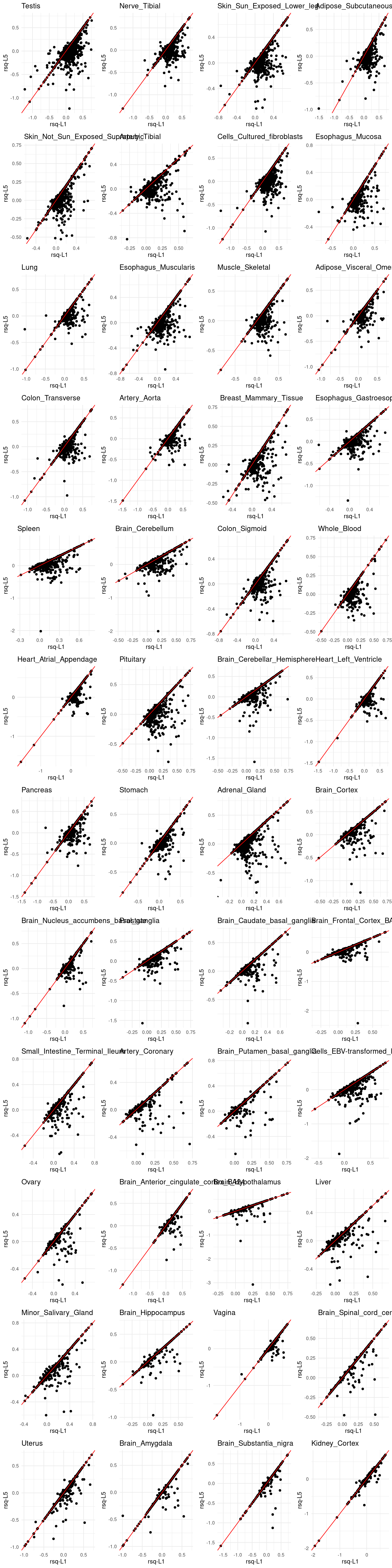

DT::datatable(sum,caption = htmltools::tags$caption( style = 'caption-side: left; text-align: left; color:black;  font-size:150% ;','Comparing L=1 & L=5'),options = list(pageLength = 10) )

Comparing with Munro’s prediction model

RNA stability – L=1

qtl = "stability"
L=1

folder_pred <-  paste0("/project/xinhe/xsun/weights_training/cv/multiplesets/",qtl,"/L",L,"/rsq_summary/")
folder_round1<- paste0("/project/xinhe/xsun/weights_training/cv/multiplesets/",qtl,"/L",L,"/round1/")

sum <- c()
for (tissue in name_mapping$Munro_name) {
  
   if(!file.exists(paste0(folder_pred,tissue,"_rsq_fusion.RDS"))) next
  
  tissue_gtex <- name_mapping$gtex_name[which(name_mapping$Munro_name == tissue)]
  
  ### our weights
  
  weights <- readRDS(paste0(folder_round1, tissue, "_training_effectsizes.RDS"))
  n_rna <- length(weights)
  
  rsq <- readRDS(paste0(folder_pred, tissue, "_rsq_fusion.RDS"))
  n_withcs <- nrow(rsq)
  n_posrsq <- sum(rsq$mean_rsq>0,na.rm = T)
  
  ### sample size 
  sample_test <- readRDS(paste0(folder_round1,tissue,"_samples_testing.RDS"))
  sample_test <- length(sample_test)
  sample_train <- readRDS(paste0(folder_round1,tissue,"_samples_training.RDS"))
  sample_train <- length(sample_train)
  sample_total <- sample_test + sample_train 
  
  ### Munro's weights
  df_munro <- read.table(paste0("/project/xinhe/xsun/weights_training/data/weights_munro/",qtl,"/",tissue,".",qtl,".twas_weights.profile"), header = T)
  n_rna_withweights_munro <- nrow(df_munro)
  ### overlap
  n_overlap_withcs <- sum(rsq$gene %in% df_munro$id)
  n_overlap_posrsq <- sum(rsq$gene[rsq$mean_rsq>0] %in% df_munro$id,na.rm=T)

  tmp_tissue <- c(tissue_gtex,sample_total,n_rna,n_rna_withweights_munro, n_withcs,n_overlap_withcs,n_posrsq,n_overlap_posrsq)
  
  sum <- rbind(sum, tmp_tissue)
}

sum <- as.data.frame(sum)
rownames(sum) <- NULL
colnames(sum) <- c("tissue","sample_size_total","n_rna_total","n_munro_weights","n_rna_withsusie_cs","overlap_cs_munro","n_rna_rsq+","overlap_rsq+_munro")

sum <- sum[order(as.numeric(sum$sample_size_total),decreasing = T),]

DT::datatable(sum,caption = htmltools::tags$caption( style = 'caption-side: left; text-align: left; color:black;  font-size:150% ;','Summary for the prediction models'),options = list(pageLength = 10) )

folder_munroweights<- paste0("/project/xinhe/xsun/weights_training/data/weights_munro/",qtl,"/")

p <- list()
for (tissue in name_mapping$Munro_name) {
  
  if(!file.exists(paste0(folder_pred,tissue,"_rsq_fusion.RDS"))) next
  
  tissue_gtex <- name_mapping$gtex_name[which(name_mapping$Munro_name == tissue)]
  
  ### our weights

  rsq <- readRDS(paste0(folder_pred, tissue, "_rsq_fusion.RDS"))
  rsq <- data.frame(id = rsq$gene, rsq = rsq$mean_rsq)
  
  ### Munro's weights
  
  summary_munro <- read.table(paste0(folder_munroweights,tissue,".",qtl,".twas_weights.profile"),header = T)
  
  merged_df <- merge(rsq, summary_munro, by= "id")
  
  p[[tissue_gtex]] <-   ggplot(merged_df, aes(x=rsq, y=lasso.r2)) + 
    geom_point() +
    labs(x = "rsq-topsnpfromsusie", y="rsq-lasso-munro") +
    geom_abline(slope = 1, intercept = 0, col="red") + 
    ggtitle(tissue_gtex) + 
    theme_minimal()

}

grid.arrange(grobs = p, ncol = 4)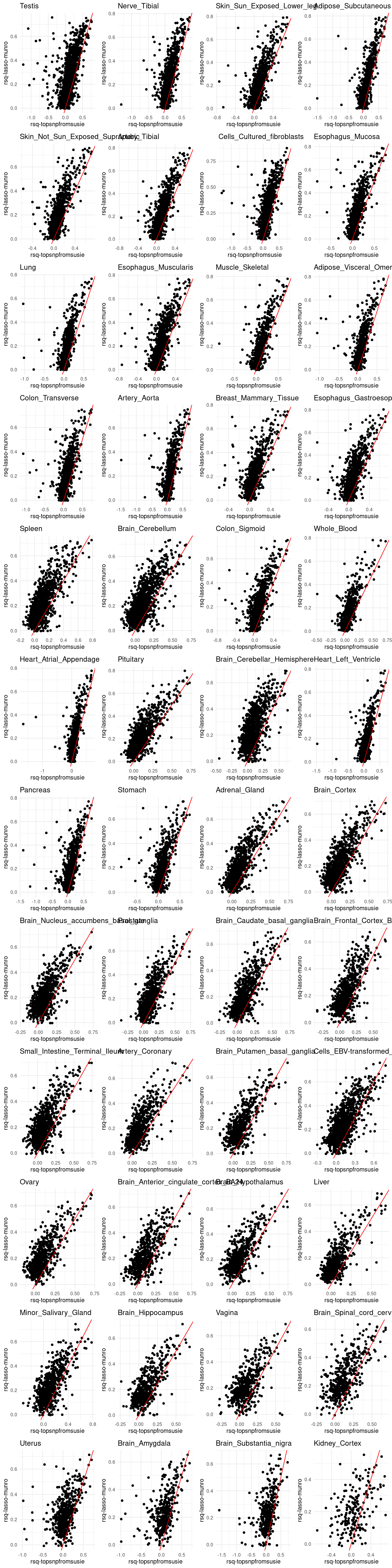

RNA stability – L=5

qtl = "stability"
L=5

folder_pred <-  paste0("/project/xinhe/xsun/weights_training/cv/multiplesets/",qtl,"/L",L,"/rsq_summary/")
folder_round1<- paste0("/project/xinhe/xsun/weights_training/cv/multiplesets/",qtl,"/L",L,"/round1/")

sum <- c()
for (tissue in name_mapping$Munro_name) {
  
   if(!file.exists(paste0(folder_pred,tissue,"_rsq_fusion.RDS"))) next
  
  tissue_gtex <- name_mapping$gtex_name[which(name_mapping$Munro_name == tissue)]
  
  ### our weights
  
  weights <- readRDS(paste0(folder_round1, tissue, "_training_effectsizes.RDS"))
  n_rna <- length(weights)
  
  rsq <- readRDS(paste0(folder_pred, tissue, "_rsq_fusion.RDS"))
  n_withcs <- nrow(rsq)
  n_posrsq <- sum(rsq$mean_rsq>0,na.rm = T)
  
  ### sample size 
  sample_test <- readRDS(paste0(folder_round1,tissue,"_samples_testing.RDS"))
  sample_test <- length(sample_test)
  sample_train <- readRDS(paste0(folder_round1,tissue,"_samples_training.RDS"))
  sample_train <- length(sample_train)
  sample_total <- sample_test + sample_train 
  
  ### Munro's weights
  df_munro <- read.table(paste0("/project/xinhe/xsun/weights_training/data/weights_munro/",qtl,"/",tissue,".",qtl,".twas_weights.profile"), header = T)
  n_rna_withweights_munro <- nrow(df_munro)
  ### overlap
  n_overlap_withcs <- sum(rsq$gene %in% df_munro$id)
  n_overlap_posrsq <- sum(rsq$gene[rsq$mean_rsq>0] %in% df_munro$id,na.rm=T)

  tmp_tissue <- c(tissue_gtex,sample_total,n_rna,n_rna_withweights_munro, n_withcs,n_overlap_withcs,n_posrsq,n_overlap_posrsq)
  
  sum <- rbind(sum, tmp_tissue)
}

sum <- as.data.frame(sum)
rownames(sum) <- NULL
colnames(sum) <- c("tissue","sample_size_total","n_rna_total","n_munro_weights","n_rna_withsusie_cs","overlap_cs_munro","n_rna_rsq+","overlap_rsq+_munro")

sum <- sum[order(as.numeric(sum$sample_size_total),decreasing = T),]

DT::datatable(sum,caption = htmltools::tags$caption( style = 'caption-side: left; text-align: left; color:black;  font-size:150% ;','Summary for the prediction models'),options = list(pageLength = 10) )

folder_munroweights<- paste0("/project/xinhe/xsun/weights_training/data/weights_munro/",qtl,"/")

p <- list()
for (tissue in name_mapping$Munro_name) {
  
  if(!file.exists(paste0(folder_pred,tissue,"_rsq_fusion.RDS"))) next
  
  tissue_gtex <- name_mapping$gtex_name[which(name_mapping$Munro_name == tissue)]
  
  ### our weights

  rsq <- readRDS(paste0(folder_pred, tissue, "_rsq_fusion.RDS"))
  rsq <- data.frame(id = rsq$gene, rsq = rsq$mean_rsq)
  
  ### Munro's weights
  
  summary_munro <- read.table(paste0(folder_munroweights,tissue,".",qtl,".twas_weights.profile"),header = T)
  
  merged_df <- merge(rsq, summary_munro, by= "id")
  
  p[[tissue_gtex]] <-   ggplot(merged_df, aes(x=rsq, y=lasso.r2)) + 
    geom_point() +
    labs(x = "rsq-topsnpfromsusie", y="rsq-lasso-munro") +
    geom_abline(slope = 1, intercept = 0, col="red") + 
    ggtitle(tissue_gtex) + 
    theme_minimal()

}

grid.arrange(grobs = p, ncol = 4)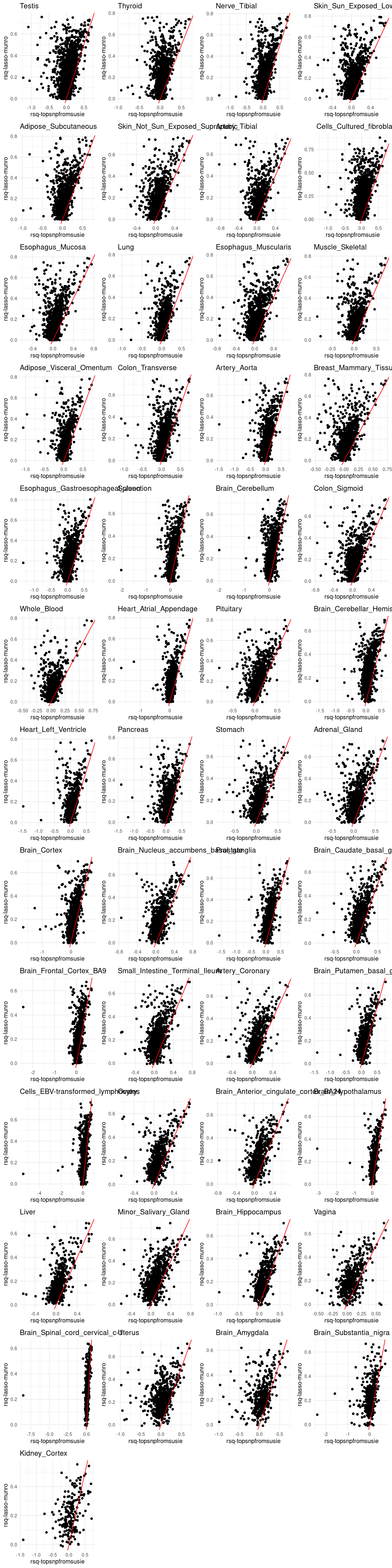

sessionInfo()

R version 4.2.0 (2022-04-22)
Platform: x86_64-pc-linux-gnu (64-bit)
Running under: CentOS Linux 7 (Core)

Matrix products: default
BLAS/LAPACK: /software/openblas-0.3.13-el7-x86_64/lib/libopenblas_haswellp-r0.3.13.so

locale:
[1] C

attached base packages:
[1] stats     graphics  grDevices utils     datasets  methods   base     

other attached packages:
[1] gridExtra_2.3 ggplot2_3.5.1 RSQLite_2.3.1

loaded via a namespace (and not attached):
 [1] tidyselect_1.2.0  xfun_0.41         bslib_0.3.1       colorspace_2.0-3 
 [5] vctrs_0.6.5       generics_0.1.2    htmltools_0.5.2   yaml_2.3.5       
 [9] utf8_1.2.2        blob_1.2.3        rlang_1.1.2       jquerylib_0.1.4  
[13] later_1.3.0       pillar_1.9.0      glue_1.6.2        withr_2.5.0      
[17] DBI_1.2.2         bit64_4.0.5       lifecycle_1.0.4   stringr_1.5.1    
[21] munsell_0.5.0     gtable_0.3.0      workflowr_1.7.0   htmlwidgets_1.5.4
[25] evaluate_0.15     memoise_2.0.1     labeling_0.4.2    knitr_1.39       
[29] fastmap_1.1.0     httpuv_1.6.5      crosstalk_1.2.0   fansi_1.0.3      
[33] highr_0.9         Rcpp_1.0.12       promises_1.2.0.1  scales_1.3.0     
[37] DT_0.22           cachem_1.0.6      jsonlite_1.8.0    farver_2.1.0     
[41] fs_1.5.2          bit_4.0.4         digest_0.6.29     stringi_1.7.6    
[45] dplyr_1.1.4       rprojroot_2.0.3   grid_4.2.0        cli_3.6.1        
[49] tools_4.2.0       magrittr_2.0.3    sass_0.4.1        tibble_3.2.1     
[53] pkgconfig_2.0.3   rmarkdown_2.25    rstudioapi_0.13   R6_2.5.1         
[57] git2r_0.30.1      compiler_4.2.0

Training stability weights using munro’s RNA data

XSun

2025-03-20