Exploring genetic architecture

workflowr

• Summary
• Checks
• Past versions

Last updated: 2025-04-29

Checks: 6 1

Knit directory: multigroup_ctwas_analysis/

This reproducible R Markdown analysis was created with workflowr (version 1.7.0). The Checks tab describes the reproducibility checks that were applied when the results were created. The Past versions tab lists the development history.

---

R Markdown file: uncommitted changes

The R Markdown file has unstaged changes. To know which version of the R Markdown file created these results, you’ll want to first commit it to the Git repo. If you’re still working on the analysis, you can ignore this warning. When you’re finished, you can run wflow_publish to commit the R Markdown file and build the HTML.

Environment: empty

Great job! The global environment was empty. Objects defined in the global environment can affect the analysis in your R Markdown file in unknown ways. For reproduciblity it’s best to always run the code in an empty environment.

Seed: set.seed(20231112)

The command set.seed(20231112) was run prior to running the code in the R Markdown file. Setting a seed ensures that any results that rely on randomness, e.g. subsampling or permutations, are reproducible.

Session information: recorded

Great job! Recording the operating system, R version, and package versions is critical for reproducibility.

Cache: none

Nice! There were no cached chunks for this analysis, so you can be confident that you successfully produced the results during this run.

File paths: relative

Great job! Using relative paths to the files within your workflowr project makes it easier to run your code on other machines.

Repository version: 3b4edbe

Great! You are using Git for version control. Tracking code development and connecting the code version to the results is critical for reproducibility.

The results in this page were generated with repository version 3b4edbe. See the Past versions tab to see a history of the changes made to the R Markdown and HTML files.

Note that you need to be careful to ensure that all relevant files for the analysis have been committed to Git prior to generating the results (you can use wflow_publish or wflow_git_commit). workflowr only checks the R Markdown file, but you know if there are other scripts or data files that it depends on. Below is the status of the Git repository when the results were generated:

Ignored files:
    Ignored:    .Rhistory
    Ignored:    cv/

Unstaged changes:
    Modified:   analysis/combine_qtls.Rmd

Note that any generated files, e.g. HTML, png, CSS, etc., are not included in this status report because it is ok for generated content to have uncommitted changes.

---

These are the previous versions of the repository in which changes were made to the R Markdown (analysis/combine_qtls.Rmd) and HTML (docs/combine_qtls.html) files. If you’ve configured a remote Git repository (see ?wflow_git_remote), click on the hyperlinks in the table below to view the files as they were in that past version.

File	Version	Author	Date	Message
Rmd	3b4edbe	XSun	2025-04-28	update
html	3b4edbe	XSun	2025-04-28	update

---

library(ctwas)
library(dplyr)
library(ggplot2)
library(ggrepel)
library(egg)
library(gridExtra)
library(grid)

#source("/project/xinhe/xsun/multi_group_ctwas/functions/0.functions.R")
source("/project/xinhe/xsun/multi_group_ctwas/data/samplesize.R")

thin <- 1
vgs <- "shared_all"
L <-5

fix_panel_size <- function(plot, width = 2.1, height = 2) {
  set_panel_size(plot, 
                 width = unit(width, "in"), 
                 height = unit(height, "in"))
}

folder_results_multiqtl <- "/project/xinhe/xsun/multi_group_ctwas/19.diff_qtls/snakemake_outputs/"

plot_piechart_topn <- function(ctwas_parameters, colors, by, title, n_tissue=10) {
  # Define fixed colors for QTL types
  qtl_colors <- c(
    eQTL = "#ff7f0e",
    sQTL = "#2ca02c",
    stQTL = "#d62728",
    edQTL = "#9467bd"
  )
  
  # Create the initial data frame
  data <- data.frame(
    category = names(ctwas_parameters$prop_heritability),
    percentage = ctwas_parameters$prop_heritability
  )
  
  # Split the category into context and type
  data <- data %>%
    mutate(
      context = sub("\\|.*", "", category),
      type = sub(".*\\|", "", category)
    )
  
  # Aggregate the data based on the 'by' parameter
  if (by == "type") {
    data <- data %>%
      group_by(type) %>%
      summarize(percentage = sum(percentage)) %>%
      mutate(category = type)
  } else if (by == "context") {
    data <- data %>%
      group_by(context) %>%
      summarize(percentage = sum(percentage)) %>%
      mutate(category = context)
  } else {
    stop("Invalid 'by' parameter. Use 'type' or 'context'.")
  }
  
  # Calculate percentage labels
  data$percentage_label <- paste0(round(data$percentage * 100, 2), "%")
  
  if(nrow(data) > (n_tissue +1)){
    data <- data %>%
      filter(context != "SNP") %>%
      arrange(desc(percentage)) %>%
      mutate(rank = row_number()) %>%
      mutate(context = ifelse(rank <= n_tissue, context, "Other_Tissues")) %>%
      group_by(context) %>%
      summarise(percentage = sum(percentage), .groups = "drop") %>%
      bind_rows(data %>% filter(context == "SNP") %>% select(context, percentage)) %>%
      mutate(
        category = context,
        percentage_label = paste0(sprintf("%.2f", percentage * 100), "%")
      ) %>%
      arrange(desc(percentage))
    
    sorted_levels <- data %>%
      mutate(sort_key = case_when(
        category == "Other_Tissues" ~ 1,
        category == "SNP" ~ 2,
        TRUE ~ 0
      )) %>%
      arrange(sort_key, desc(percentage)) %>%
      pull(category)
  } else {
    sorted_levels <- data %>%
      arrange((category == "SNP"), desc(percentage)) %>%
      pull(category)
  }
  
  data$category <- factor(data$category, levels = sorted_levels)
  
  # Order data for positioning
  data <- data %>% 
    arrange(category) %>%
    mutate(
      cumulative = cumsum(percentage),
      midpoint = cumulative - percentage / 2
    )
  
  # Prepare colors
  categories <- levels(data$category)
  has_snp <- "SNP" %in% categories
  other_cats <- setdiff(categories, "SNP")
  
  color_vec <- c()
  if (has_snp) color_vec["SNP"] <- "#1f77b4"
  
  # Split categories into QTL and non-QTL
  qtl_cats <- other_cats[other_cats %in% names(qtl_colors)]
  non_qtl_cats <- other_cats[!other_cats %in% names(qtl_colors)]
  
  # Assign QTL colors
  for (cat in qtl_cats) color_vec[cat] <- qtl_colors[cat]
  
  # Assign non-QTL colors
  if (length(non_qtl_cats) > 0) {
    if (is.null(names(colors))) {
      colors_non_qtl <- rep(colors, length.out = length(non_qtl_cats))
      color_vec <- c(color_vec, setNames(colors_non_qtl, non_qtl_cats))
    } else {
      for (cat in non_qtl_cats) {
        color_vec[cat] <- ifelse(cat %in% names(colors), colors[cat], "#808080")
      }
    }
  }
  
  # Calculate label positions
  data <- data %>%
    mutate(
      y_pos = midpoint,
      angle = 0,
      hjust = 0.5
    )
  
  # Create pie chart
  pie <- ggplot(data, aes(x = "", y = percentage, fill = category)) +
    geom_bar(stat = "identity", width = 1) +
    coord_polar("y", start = 0) +
    theme_void() +
    geom_text_repel(
      aes(
        y = 1 - y_pos,
        label = percentage_label,
        angle = angle
      ),
      size = 3,
      nudge_x = 0.8,
      segment.size = 0.3,
      segment.color = "gray40",
      box.padding = 0.2,
      min.segment.length = 0.1,
      hjust = 0.5,
      vjust = 0.5
    ) +
    scale_fill_manual(values = color_vec) +
    labs(fill = "") +
    ggtitle(title)
  
  return(pie)
}

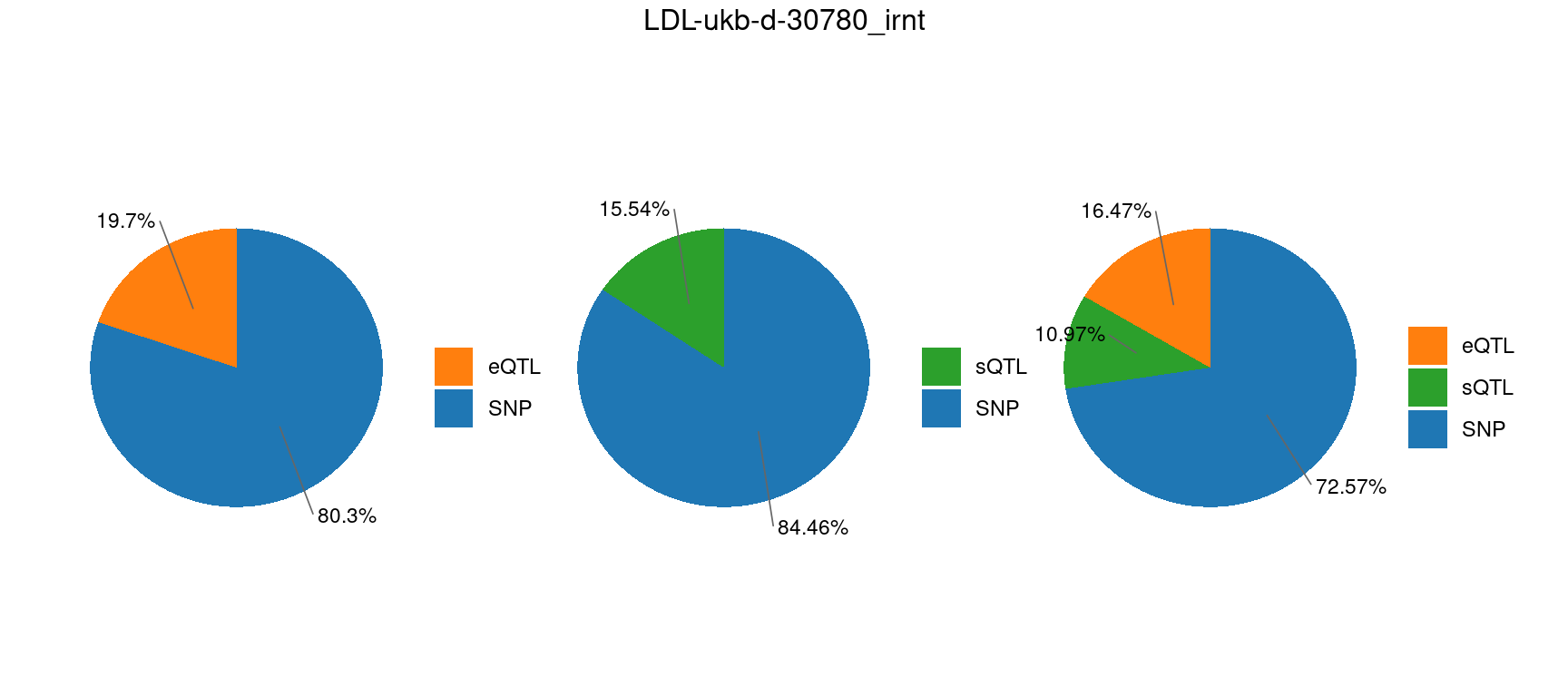
LDL-ukb-d-30780_irnt, Liver

trait <- "LDL-ukb-d-30780_irnt"

gwas_n <- samplesize[trait]

Comparing eQTL, sQTL and eQTL + sQTL

qtl <- "eonly"

file_param <- paste0(folder_results_multiqtl, trait, "/", trait, ".", qtl, ".thin", thin, ".", vgs, ".param.RDS")
param <- readRDS(file_param)
ctwas_parameters <- summarize_param(param, gwas_n)

p1 <- plot_piechart_topn(ctwas_parameters = ctwas_parameters,colors = colors,by = "type",title = NULL)

qtl <- "sonly"

file_param <- paste0(folder_results_multiqtl, trait, "/", trait, ".", qtl, ".thin", thin, ".", vgs, ".param.RDS")
param <- readRDS(file_param)
ctwas_parameters <- summarize_param(param, gwas_n)

p2 <- plot_piechart_topn(ctwas_parameters = ctwas_parameters,colors = colors,by = "type",title = NULL)

qtl <- "es"

file_param <- paste0(folder_results_multiqtl, trait, "/", trait, ".", qtl, ".thin", thin, ".", vgs, ".param.RDS")
param <- readRDS(file_param)
ctwas_parameters <- summarize_param(param, gwas_n)

p3 <- plot_piechart_topn(ctwas_parameters = ctwas_parameters,colors = colors,by = "type",title = NULL)


# Convert plots to gtables with fixed panel sizes
pie1 <- fix_panel_size(p1)
pie2 <- fix_panel_size(p2)
pie3 <- fix_panel_size(p3)

# Calculate widths of each gtable (plot + legend)
widths <- unit.c(grobWidth(pie1), grobWidth(pie2), grobWidth(pie3))

# Arrange plots with their natural widths
p <- grid.arrange(pie1, pie2, pie3, 
                  ncol = 3, 
                  widths = widths,
                  top = paste0(trait)
)

Past versions of unnamed-chunk-3-1.png

Version	Author	Date
3b4edbe	XSun	2025-04-28

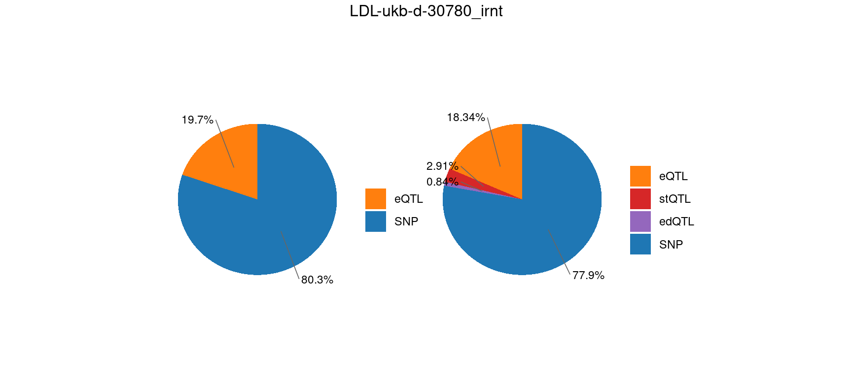
Comparing eQTL and eQTL + stQTL + edQTL

qtl <- "eonly"

file_param <- paste0(folder_results_multiqtl, trait, "/", trait, ".", qtl, ".thin", thin, ".", vgs, ".param.RDS")
param <- readRDS(file_param)
ctwas_parameters <- summarize_param(param, gwas_n)

p1 <- plot_piechart_topn(ctwas_parameters = ctwas_parameters,colors = colors,by = "type",title = NULL)

qtl <- "ested"

file_param <- paste0(folder_results_multiqtl, trait, "/", trait, ".", qtl, ".thin", thin, ".", vgs, ".param.RDS")
param <- readRDS(file_param)
ctwas_parameters <- summarize_param(param, gwas_n)

p2 <- plot_piechart_topn(ctwas_parameters = ctwas_parameters,colors = colors,by = "type",title = NULL)


pie1 <- fix_panel_size(p1)
pie2 <- fix_panel_size(p2)

# Calculate widths of each gtable (plot + legend)
widths <- unit.c(grobWidth(pie1), grobWidth(pie2))

# Arrange plots with their natural widths
p <- grid.arrange(pie1, pie2,  
                  ncol = 2, 
                  widths = widths,
                  top = paste0(trait)
)

Past versions of unnamed-chunk-4-1.png

Version	Author	Date
3b4edbe	XSun	2025-04-28

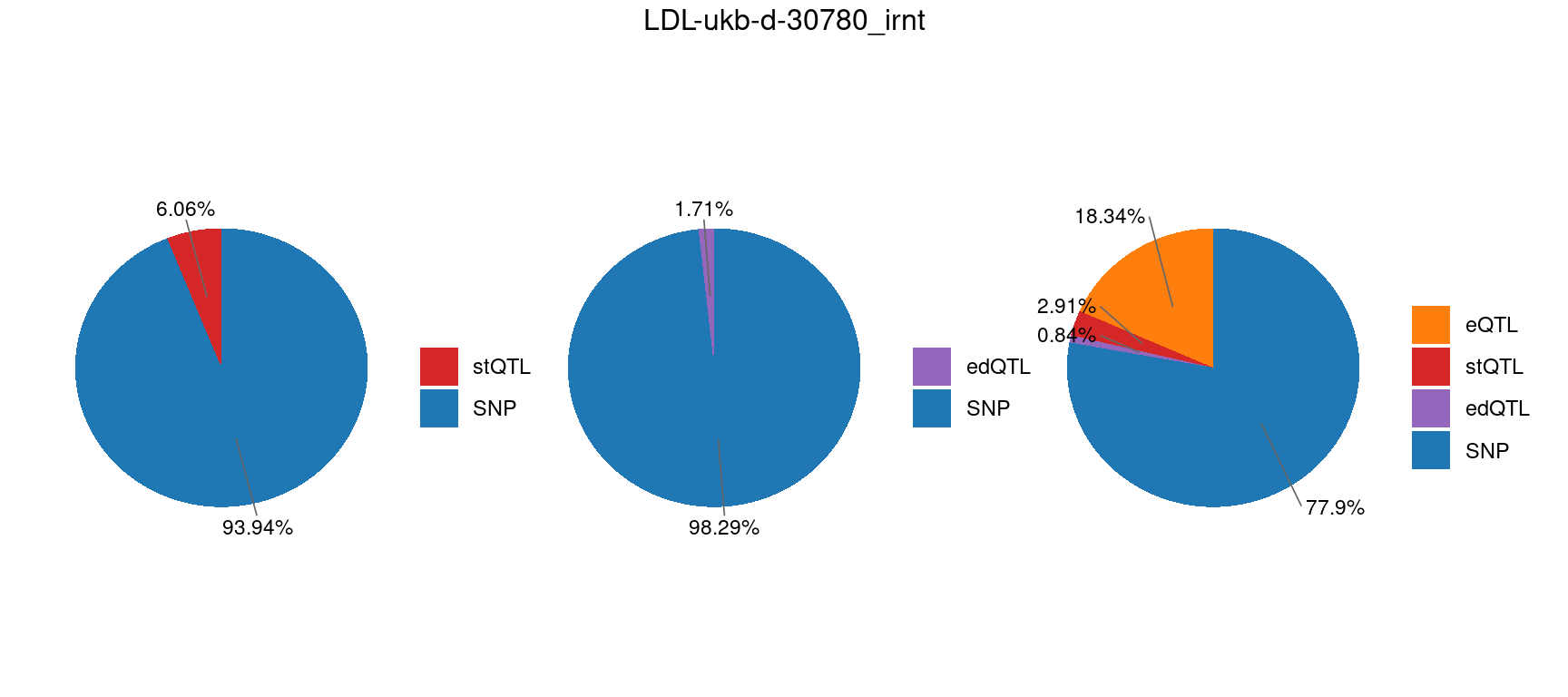
Comparing stQTL, edQTL and eQTL + stQTL + edQTL

qtl <- "stonly"

file_param <- paste0(folder_results_multiqtl, trait, "/", trait, ".", qtl, ".thin", thin, ".", vgs, ".param.RDS")
param <- readRDS(file_param)
ctwas_parameters <- summarize_param(param, gwas_n)

p1 <- plot_piechart_topn(ctwas_parameters = ctwas_parameters,colors = colors,by = "type",title = NULL)

qtl <- "edonly"

file_param <- paste0(folder_results_multiqtl, trait, "/", trait, ".", qtl, ".thin", thin, ".", vgs, ".param.RDS")
param <- readRDS(file_param)
ctwas_parameters <- summarize_param(param, gwas_n)

p2 <- plot_piechart_topn(ctwas_parameters = ctwas_parameters,colors = colors,by = "type",title = NULL)

qtl <- "ested"

file_param <- paste0(folder_results_multiqtl, trait, "/", trait, ".", qtl, ".thin", thin, ".", vgs, ".param.RDS")
param <- readRDS(file_param)
ctwas_parameters <- summarize_param(param, gwas_n)

p3 <- plot_piechart_topn(ctwas_parameters = ctwas_parameters,colors = colors,by = "type",title = NULL)


# Convert plots to gtables with fixed panel sizes
pie1 <- fix_panel_size(p1)
pie2 <- fix_panel_size(p2)
pie3 <- fix_panel_size(p3)

# Calculate widths of each gtable (plot + legend)
widths <- unit.c(grobWidth(pie1), grobWidth(pie2), grobWidth(pie3))

# Arrange plots with their natural widths
p <- grid.arrange(pie1, pie2, pie3, 
                  ncol = 3, 
                  widths = widths,
                  top = paste0(trait)
)

Past versions of unnamed-chunk-5-1.png

Version	Author	Date
3b4edbe	XSun	2025-04-28

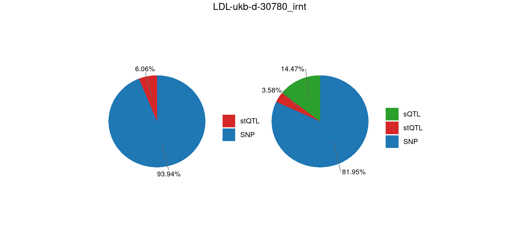
Comparing stQTL and stQTL + sQTL

qtl <- "stonly"

file_param <- paste0(folder_results_multiqtl, trait, "/", trait, ".", qtl, ".thin", thin, ".", vgs, ".param.RDS")
param <- readRDS(file_param)
ctwas_parameters <- summarize_param(param, gwas_n)

p1 <- plot_piechart_topn(ctwas_parameters = ctwas_parameters,colors = colors,by = "type",title = NULL)

qtl <- "sts"

file_param <- paste0(folder_results_multiqtl, trait, "/", trait, ".", qtl, ".thin", thin, ".", vgs, ".param.RDS")
param <- readRDS(file_param)
ctwas_parameters <- summarize_param(param, gwas_n)

p2 <- plot_piechart_topn(ctwas_parameters = ctwas_parameters,colors = colors,by = "type",title = NULL)


pie1 <- fix_panel_size(p1)
pie2 <- fix_panel_size(p2)

# Calculate widths of each gtable (plot + legend)
widths <- unit.c(grobWidth(pie1), grobWidth(pie2))

# Arrange plots with their natural widths
p <- grid.arrange(pie1, pie2,  
                  ncol = 2, 
                  widths = widths,
                  top = paste0(trait)
)

Past versions of unnamed-chunk-6-1.png

Version	Author	Date
3b4edbe	XSun	2025-04-28

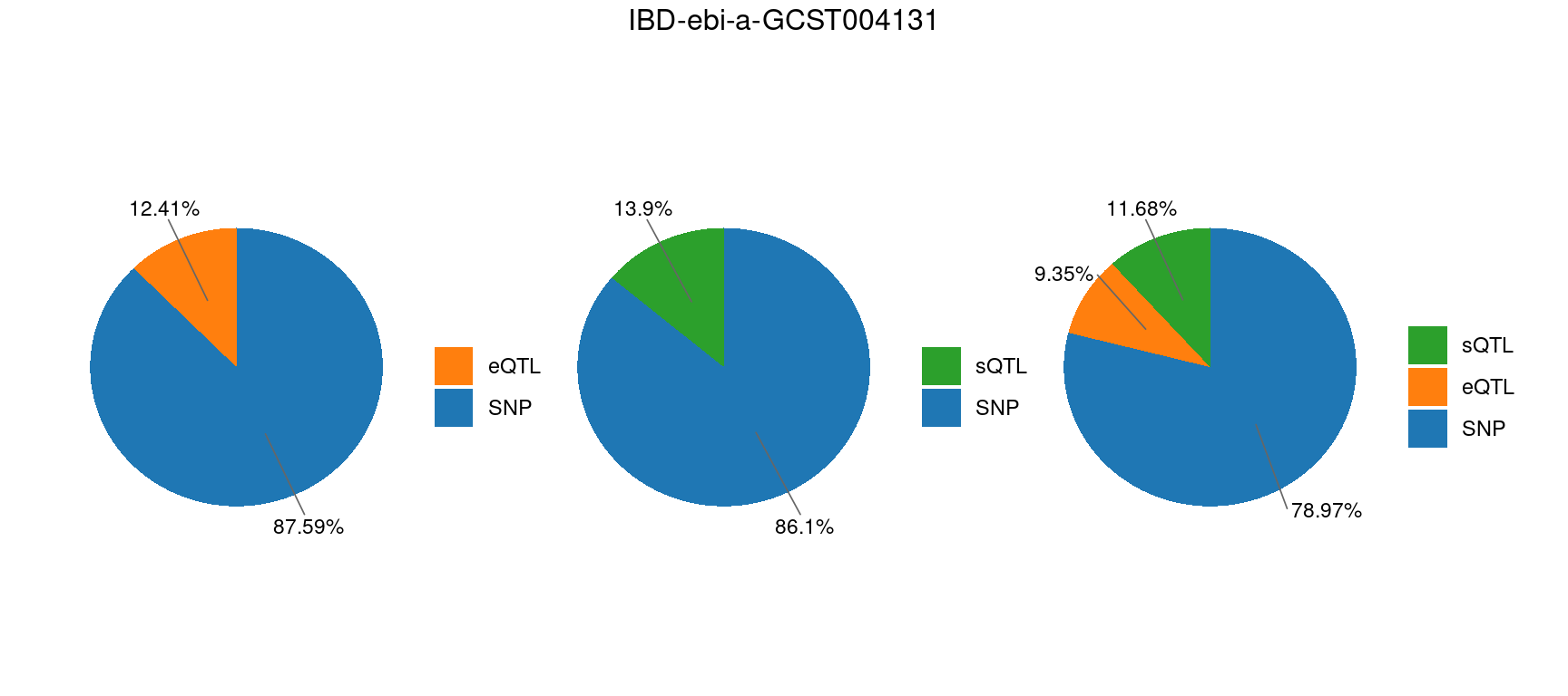
IBD-ebi-a-GCST004131, Whole_Blood & Colon_Transverse

trait <- "IBD-ebi-a-GCST004131"

gwas_n <- samplesize[trait]

Comparing eQTL, sQTL and eQTL + sQTL

qtl <- "eonly"

file_param <- paste0(folder_results_multiqtl, trait, "/", trait, ".", qtl, ".thin", thin, ".", vgs, ".param.RDS")
param <- readRDS(file_param)
ctwas_parameters <- summarize_param(param, gwas_n)

p1 <- plot_piechart_topn(ctwas_parameters = ctwas_parameters,colors = colors,by = "type",title = NULL)

qtl <- "sonly"

file_param <- paste0(folder_results_multiqtl, trait, "/", trait, ".", qtl, ".thin", thin, ".", vgs, ".param.RDS")
param <- readRDS(file_param)
ctwas_parameters <- summarize_param(param, gwas_n)

p2 <- plot_piechart_topn(ctwas_parameters = ctwas_parameters,colors = colors,by = "type",title = NULL)

qtl <- "es"

file_param <- paste0(folder_results_multiqtl, trait, "/", trait, ".", qtl, ".thin", thin, ".", vgs, ".param.RDS")
param <- readRDS(file_param)
ctwas_parameters <- summarize_param(param, gwas_n)

p3 <- plot_piechart_topn(ctwas_parameters = ctwas_parameters,colors = colors,by = "type",title = NULL)


# Convert plots to gtables with fixed panel sizes
pie1 <- fix_panel_size(p1)
pie2 <- fix_panel_size(p2)
pie3 <- fix_panel_size(p3)

# Calculate widths of each gtable (plot + legend)
widths <- unit.c(grobWidth(pie1), grobWidth(pie2), grobWidth(pie3))

# Arrange plots with their natural widths
p <- grid.arrange(pie1, pie2, pie3, 
                  ncol = 3, 
                  widths = widths,
                  top = paste0(trait)
)

Past versions of unnamed-chunk-8-1.png

Version	Author	Date
3b4edbe	XSun	2025-04-28

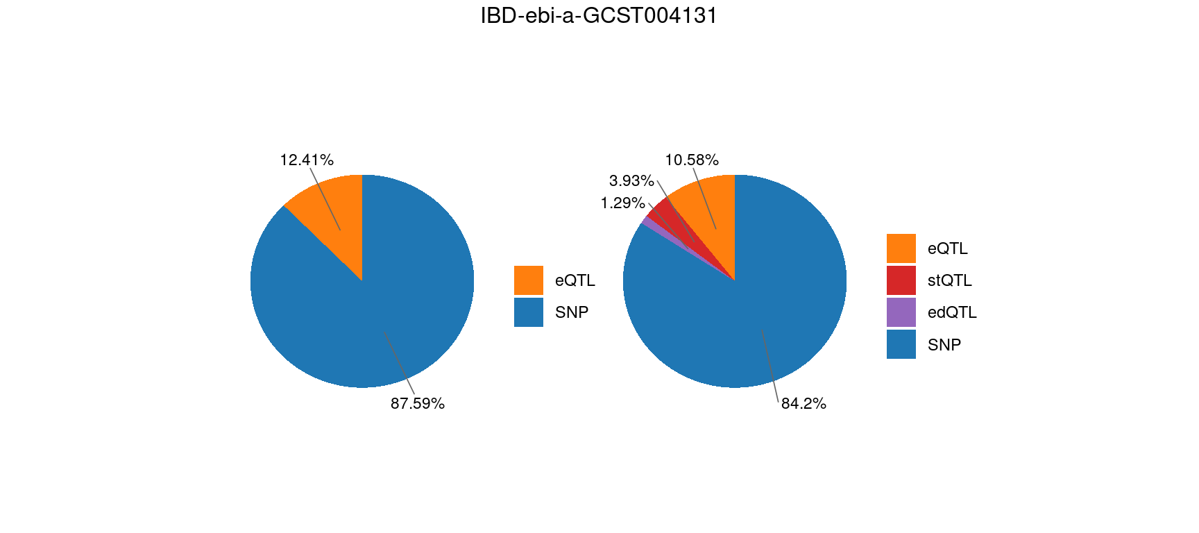
Comparing eQTL and eQTL + stQTL + edQTL

qtl <- "eonly"

file_param <- paste0(folder_results_multiqtl, trait, "/", trait, ".", qtl, ".thin", thin, ".", vgs, ".param.RDS")
param <- readRDS(file_param)
ctwas_parameters <- summarize_param(param, gwas_n)

p1 <- plot_piechart_topn(ctwas_parameters = ctwas_parameters,colors = colors,by = "type",title = NULL)

qtl <- "ested"

file_param <- paste0(folder_results_multiqtl, trait, "/", trait, ".", qtl, ".thin", thin, ".", vgs, ".param.RDS")
param <- readRDS(file_param)
ctwas_parameters <- summarize_param(param, gwas_n)

p2 <- plot_piechart_topn(ctwas_parameters = ctwas_parameters,colors = colors,by = "type",title = NULL)


pie1 <- fix_panel_size(p1)
pie2 <- fix_panel_size(p2)

# Calculate widths of each gtable (plot + legend)
widths <- unit.c(grobWidth(pie1), grobWidth(pie2))

# Arrange plots with their natural widths
p <- grid.arrange(pie1, pie2,  
                  ncol = 2, 
                  widths = widths,
                  top = paste0(trait)
)

Past versions of unnamed-chunk-9-1.png

Version	Author	Date
3b4edbe	XSun	2025-04-28

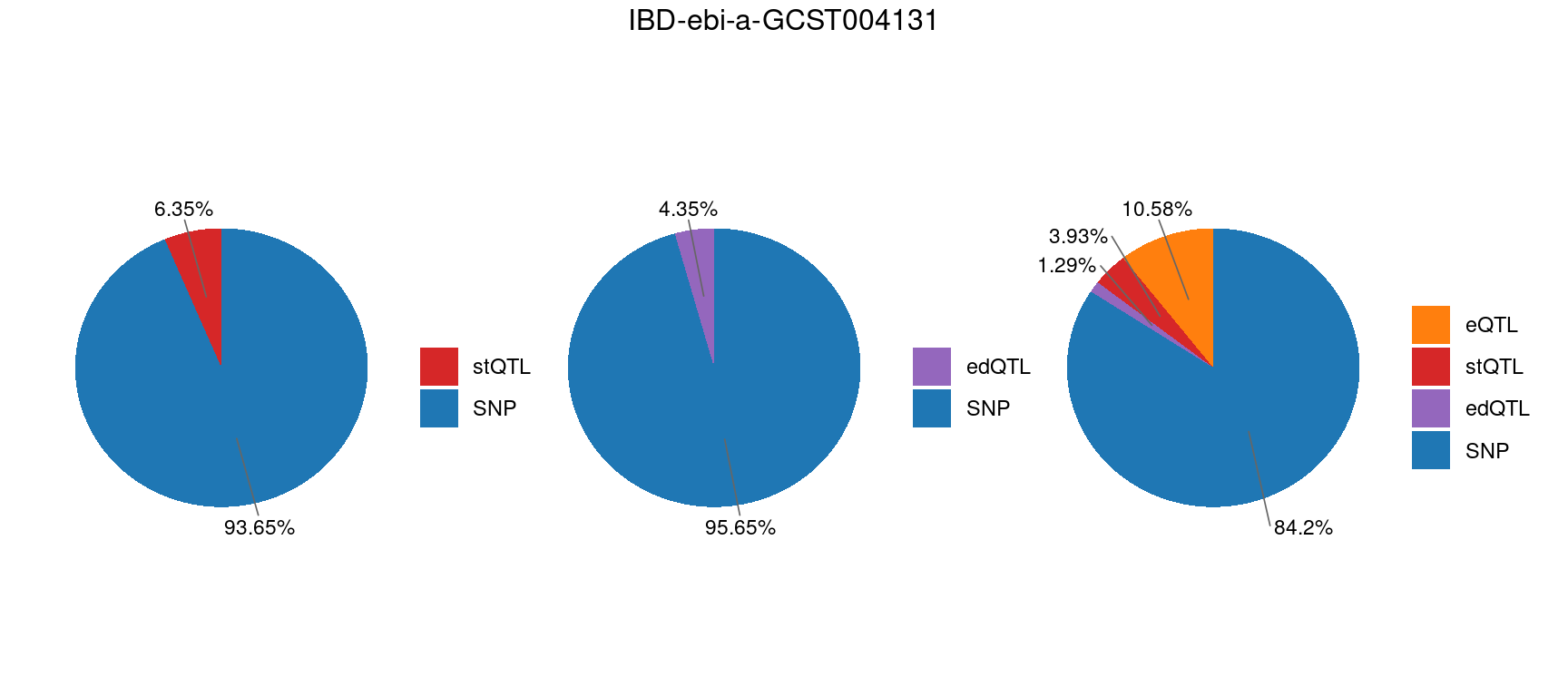
Comparing stQTL, edQTL and eQTL + stQTL + edQTL

qtl <- "stonly"

file_param <- paste0(folder_results_multiqtl, trait, "/", trait, ".", qtl, ".thin", thin, ".", vgs, ".param.RDS")
param <- readRDS(file_param)
ctwas_parameters <- summarize_param(param, gwas_n)

p1 <- plot_piechart_topn(ctwas_parameters = ctwas_parameters,colors = colors,by = "type",title = NULL)

qtl <- "edonly"

file_param <- paste0(folder_results_multiqtl, trait, "/", trait, ".", qtl, ".thin", thin, ".", vgs, ".param.RDS")
param <- readRDS(file_param)
ctwas_parameters <- summarize_param(param, gwas_n)

p2 <- plot_piechart_topn(ctwas_parameters = ctwas_parameters,colors = colors,by = "type",title = NULL)

qtl <- "ested"

file_param <- paste0(folder_results_multiqtl, trait, "/", trait, ".", qtl, ".thin", thin, ".", vgs, ".param.RDS")
param <- readRDS(file_param)
ctwas_parameters <- summarize_param(param, gwas_n)

p3 <- plot_piechart_topn(ctwas_parameters = ctwas_parameters,colors = colors,by = "type",title = NULL)


# Convert plots to gtables with fixed panel sizes
pie1 <- fix_panel_size(p1)
pie2 <- fix_panel_size(p2)
pie3 <- fix_panel_size(p3)

# Calculate widths of each gtable (plot + legend)
widths <- unit.c(grobWidth(pie1), grobWidth(pie2), grobWidth(pie3))

# Arrange plots with their natural widths
p <- grid.arrange(pie1, pie2, pie3, 
                  ncol = 3, 
                  widths = widths,
                  top = paste0(trait)
)

Past versions of unnamed-chunk-10-1.png

Version	Author	Date
3b4edbe	XSun	2025-04-28

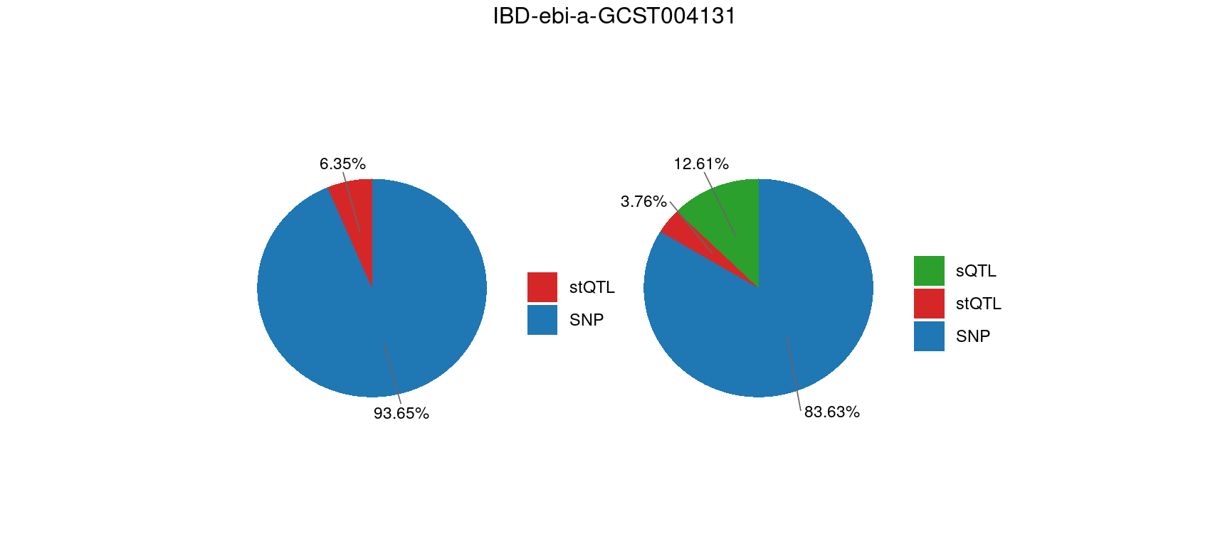
Comparing stQTL and stQTL + sQTL

qtl <- "stonly"

file_param <- paste0(folder_results_multiqtl, trait, "/", trait, ".", qtl, ".thin", thin, ".", vgs, ".param.RDS")
param <- readRDS(file_param)
ctwas_parameters <- summarize_param(param, gwas_n)

p1 <- plot_piechart_topn(ctwas_parameters = ctwas_parameters,colors = colors,by = "type",title = NULL)

qtl <- "sts"

file_param <- paste0(folder_results_multiqtl, trait, "/", trait, ".", qtl, ".thin", thin, ".", vgs, ".param.RDS")
param <- readRDS(file_param)
ctwas_parameters <- summarize_param(param, gwas_n)

p2 <- plot_piechart_topn(ctwas_parameters = ctwas_parameters,colors = colors,by = "type",title = NULL)


pie1 <- fix_panel_size(p1)
pie2 <- fix_panel_size(p2)

# Calculate widths of each gtable (plot + legend)
widths <- unit.c(grobWidth(pie1), grobWidth(pie2))

# Arrange plots with their natural widths
p <- grid.arrange(pie1, pie2,  
                  ncol = 2, 
                  widths = widths,
                  top = paste0(trait)
)

Past versions of unnamed-chunk-11-1.png

Version	Author	Date
3b4edbe	XSun	2025-04-28

Session information

sessionInfo()

R version 4.2.0 (2022-04-22)
Platform: x86_64-pc-linux-gnu (64-bit)
Running under: CentOS Linux 7 (Core)

Matrix products: default
BLAS/LAPACK: /software/openblas-0.3.13-el7-x86_64/lib/libopenblas_haswellp-r0.3.13.so

locale:
[1] C

attached base packages:
[1] grid      stats     graphics  grDevices utils     datasets  methods  
[8] base     

other attached packages:
[1] egg_0.4.5        gridExtra_2.3    ggrepel_0.9.1    ggplot2_3.5.1   
[5] dplyr_1.1.4      ctwas_0.5.4.9000

loaded via a namespace (and not attached):
  [1] colorspace_2.0-3            rjson_0.2.21               
  [3] ellipsis_0.3.2              rprojroot_2.0.3            
  [5] XVector_0.36.0              locuszoomr_0.2.1           
  [7] GenomicRanges_1.48.0        base64enc_0.1-3            
  [9] fs_1.5.2                    rstudioapi_0.13            
 [11] farver_2.1.0                bit64_4.0.5                
 [13] AnnotationDbi_1.58.0        fansi_1.0.3                
 [15] xml2_1.3.3                  codetools_0.2-18           
 [17] logging_0.10-108            cachem_1.0.6               
 [19] knitr_1.39                  jsonlite_1.8.0             
 [21] workflowr_1.7.0             Rsamtools_2.12.0           
 [23] dbplyr_2.1.1                png_0.1-7                  
 [25] readr_2.1.2                 compiler_4.2.0             
 [27] httr_1.4.3                  assertthat_0.2.1           
 [29] Matrix_1.5-3                fastmap_1.1.0              
 [31] lazyeval_0.2.2              cli_3.6.1                  
 [33] later_1.3.0                 htmltools_0.5.2            
 [35] prettyunits_1.1.1           tools_4.2.0                
 [37] gtable_0.3.0                glue_1.6.2                 
 [39] GenomeInfoDbData_1.2.8      rappdirs_0.3.3             
 [41] Rcpp_1.0.12                 Biobase_2.56.0             
 [43] jquerylib_0.1.4             vctrs_0.6.5                
 [45] Biostrings_2.64.0           rtracklayer_1.56.0         
 [47] xfun_0.41                   stringr_1.5.1              
 [49] irlba_2.3.5                 lifecycle_1.0.4            
 [51] restfulr_0.0.14             ensembldb_2.20.2           
 [53] XML_3.99-0.14               zlibbioc_1.42.0            
 [55] zoo_1.8-10                  scales_1.3.0               
 [57] gggrid_0.2-0                hms_1.1.1                  
 [59] promises_1.2.0.1            MatrixGenerics_1.8.0       
 [61] ProtGenerics_1.28.0         parallel_4.2.0             
 [63] SummarizedExperiment_1.26.1 AnnotationFilter_1.20.0    
 [65] LDlinkR_1.2.3               yaml_2.3.5                 
 [67] curl_4.3.2                  memoise_2.0.1              
 [69] sass_0.4.1                  biomaRt_2.54.1             
 [71] stringi_1.7.6               RSQLite_2.3.1              
 [73] highr_0.9                   S4Vectors_0.34.0           
 [75] BiocIO_1.6.0                GenomicFeatures_1.48.3     
 [77] BiocGenerics_0.42.0         filelock_1.0.2             
 [79] BiocParallel_1.30.3         repr_1.1.4                 
 [81] GenomeInfoDb_1.39.9         rlang_1.1.2                
 [83] pkgconfig_2.0.3             matrixStats_0.62.0         
 [85] bitops_1.0-7                evaluate_0.15              
 [87] lattice_0.20-45             purrr_1.0.2                
 [89] labeling_0.4.2              GenomicAlignments_1.32.0   
 [91] htmlwidgets_1.5.4           cowplot_1.1.1              
 [93] bit_4.0.4                   tidyselect_1.2.0           
 [95] magrittr_2.0.3              AMR_2.1.1                  
 [97] R6_2.5.1                    IRanges_2.30.0             
 [99] generics_0.1.2              DelayedArray_0.22.0        
[101] DBI_1.2.2                   withr_2.5.0                
[103] pgenlibr_0.3.3              pillar_1.9.0               
[105] whisker_0.4                 mixsqp_0.3-43              
[107] KEGGREST_1.36.3             RCurl_1.98-1.7             
[109] tibble_3.2.1                crayon_1.5.1               
[111] utf8_1.2.2                  BiocFileCache_2.4.0        
[113] plotly_4.10.0               tzdb_0.4.0                 
[115] rmarkdown_2.25              progress_1.2.2             
[117] data.table_1.14.2           blob_1.2.3                 
[119] git2r_0.30.1                digest_0.6.29              
[121] tidyr_1.3.0                 httpuv_1.6.5               
[123] stats4_4.2.0                munsell_0.5.0              
[125] viridisLite_0.4.0           skimr_2.1.4                
[127] bslib_0.3.1