cTWAS results from analysis of LDL GWAS
XSun
2024-10-10
Last updated: 2024-10-14
Checks: 6 1
Knit directory: multigroup_ctwas_analysis/
This reproducible R Markdown analysis was created with workflowr (version 1.7.0). The Checks tab describes the reproducibility checks that were applied when the results were created. The Past versions tab lists the development history.
The R Markdown file has unstaged changes. To know which version of
the R Markdown file created these results, you’ll want to first commit
it to the Git repo. If you’re still working on the analysis, you can
ignore this warning. When you’re finished, you can run
wflow_publish to commit the R Markdown file and build the
HTML.
Great job! The global environment was empty. Objects defined in the global environment can affect the analysis in your R Markdown file in unknown ways. For reproduciblity it’s best to always run the code in an empty environment.
The command set.seed(20231112) was run prior to running
the code in the R Markdown file. Setting a seed ensures that any results
that rely on randomness, e.g. subsampling or permutations, are
reproducible.
Great job! Recording the operating system, R version, and package versions is critical for reproducibility.
Nice! There were no cached chunks for this analysis, so you can be confident that you successfully produced the results during this run.
Great job! Using relative paths to the files within your workflowr project makes it easier to run your code on other machines.
Great! You are using Git for version control. Tracking code development and connecting the code version to the results is critical for reproducibility.
The results in this page were generated with repository version 92d55dd. See the Past versions tab to see a history of the changes made to the R Markdown and HTML files.
Note that you need to be careful to ensure that all relevant files for
the analysis have been committed to Git prior to generating the results
(you can use wflow_publish or
wflow_git_commit). workflowr only checks the R Markdown
file, but you know if there are other scripts or data files that it
depends on. Below is the status of the Git repository when the results
were generated:
Ignored files:
    Ignored:    .Rhistory

Unstaged changes:
    Modified:   analysis/LDL_predictdb_esQTL.Rmd
    Modified:   analysis/fractional_enrichment_LDL_es.Rmd
Note that any generated files, e.g. HTML, png, CSS, etc., are not included in this status report because it is ok for generated content to have uncommitted changes.
These are the previous versions of the repository in which changes were
made to the R Markdown (analysis/LDL_predictdb_esQTL.Rmd)
and HTML (docs/LDL_predictdb_esQTL.html) files. If you’ve
configured a remote Git repository (see ?wflow_git_remote),
click on the hyperlinks in the table below to view the files as they
were in that past version.
| File | Version | Author | Date | Message |
|---|---|---|---|---|
| Rmd | 04a6e93 | XSun | 2024-10-10 | update |
| html | 04a6e93 | XSun | 2024-10-10 | update |
| Rmd | 03f2e81 | XSun | 2024-09-30 | update |
| Rmd | a9f905d | sq-96 | 2024-09-30 | update |
| html | a9f905d | sq-96 | 2024-09-30 | update |
| Rmd | 7f5dfdf | GitHub | 2024-09-30 | Delete analysis/LDL_predictdb_esQTL.Rmd |
| Rmd | d450a77 | XSun | 2024-09-30 | update |
| Rmd | 6cf9e49 | XSun | 2024-09-30 | update |
| html | 6cf9e49 | XSun | 2024-09-30 | update |
| Rmd | dcdeacb | XSun | 2024-09-28 | update |
| html | dcdeacb | XSun | 2024-09-28 | update |
| Rmd | 278395e | XSun | 2024-09-24 | update |
| html | 278395e | XSun | 2024-09-24 | update |
We present a sample cTWAS report based on real data analysis. The analyzed trait is LDL cholesterol, the prediction models are liver gene expression and splicing models trained on GTEx v8 in the PredictDB format.
Analysis settings
Input data
- GWAS Z-scores
The summary statistics for LDL are downloaded from https://gwas.mrcieu.ac.uk, using dataset ID:
ukb-d-30780_irnt. The number of SNPs it contains is
13,586,016.
The sample size is
[1] "gwas_n = 343621"- Prediction models
The prediction models used in this analysis are liver gene expression and splicing models, trained on GTEx v8 in the PredictDB format. These models can be downloaded from https://predictdb.org/post/2021/07/21/gtex-v8-models-on-eqtl-and-sqtl/
[1] "The number of eQTLs per gene = 1.5078"[1] "Total number of genes = 12714"[1] "The number of sQTLs per intron = 1.2151"[1] "Total number of introns = 29250"- Reference data
The reference data include genomic region definitions and an LD
reference. We use the genomic regions provided by the package and the LD
reference in b38, located in RCC cluster of UChicago:
/project2/mstephens/wcrouse/UKB_LDR_0.1/. Alternatively,
the LD reference can be downloaded from this link:https://uchicago.app.box.com/s/jqocacd2fulskmhoqnasrknbt59x3xkn.
Data processing and harmonization
We map the reference SNPs and LD matrices to regions following the instructions from the cTWAS tutorial.
When processing z-scores, we exclude multi-allelic and
strand-ambiguous variants by setting
drop_multiallelic = TRUE and
drop_strand_ambig = TRUE.
The process can be divided into steps below, users can expand the code snippets below to view the exact code used.
- Input and output settings
weight_files <- c("/project2/xinhe/shared_data/multigroup_ctwas/weights/expression_models/expression_Liver.db","/project2/xinhe/shared_data/multigroup_ctwas/weights/splicing_models/splicing_Liver.db")
z_snp_file <- "/project2/xinhe/shared_data/multigroup_ctwas/gwas/ctwas_inputs_zsnp/LDL-ukb-d-30780_irnt.z_snp.RDS"
genome_version <- "b38"
LD_dir <- "/project2/mstephens/wcrouse/UKB_LDR_0.1/"
region_file <- system.file("extdata/ldetect", paste0("EUR.", genome_version, ".ldetect.regions.RDS"), package = "ctwas")
region_info <- readRDS(region_file)

## output dir
outputdir <- "/project/xinhe/xsun/multi_group_ctwas/examples/results_predictdb_main/LDL-ukb-d-30780_irnt/"
dir.create(outputdir, showWarnings=F, recursive=T)

## other parameters
ncore <- 5- Preprocessing GWAS
### Preprocess LD_map & SNP_map
region_metatable <- region_info
region_metatable$LD_file <- file.path(LD_dir, paste0(LD_filestem, ".RDS"))
region_metatable$SNP_file <- file.path(LD_dir, paste0(LD_filestem, ".Rvar"))

res <- create_snp_LD_map(region_metatable)

region_info <- res$region_info
snp_map <- res$snp_map
LD_map <- res$LD_map

### Preprocess GWAS z-scores
z_snp <- readRDS(z_snp_file)
z_snp <- preprocess_z_snp(z_snp = z_snp,
                          snp_map = snp_map,
                          drop_multiallelic = TRUE,
drop_strand_ambig = TRUE)- Preprocessing weights
weights_expression1 <- preprocess_weights(weight_file = weight_files[1],
                                              region_info = region_info,
                                              gwas_snp_ids = z_snp$id,
                                              snp_map = snp_map,
                                              LD_map = LD_map,
                                              type = "eQTL",
                                              context = tissue,
                                              weight_format = "PredictDB",
                                              drop_strand_ambig = TRUE,
                                              scale_predictdb_weights = T, #### F for fusion converted weights
                                              load_predictdb_LD = F, #### F for fusion converted weights or want to compute LD from LD reference
                                              filter_protein_coding_genes = TRUE,
                                              ncore = ncore)

weights_splicing1 <- preprocess_weights(weight_file = weight_files[2],
                                            region_info = region_info,
                                            gwas_snp_ids = z_snp$id,
                                            snp_map = snp_map,
                                            LD_map = LD_map,
                                            type = "sQTL",
                                            context = tissue,
                                            weight_format = "PredictDB",
                                            drop_strand_ambig = TRUE,
                                            scale_predictdb_weights = T, #### F for fusion converted weights
                                            load_predictdb_LD = F,  #### F for fusion converted weights or want to compute LD from LD reference
                                            filter_protein_coding_genes = TRUE,
                                            ncore = ncore)

weights <- c(weights_expression1,weights_splicing1)
Running cTWAS analysis
We use the ctwas main function ctwas_sumstats() to run
the cTWAS analysis with LD. For more details on this function, refer to
the cTWAS tutorial: https://xinhe-lab.github.io/multigroup_ctwas/articles/running_ctwas_analysis.html#running-ctwas-main-function
All arguments are set to their default values, with the following specific settings:
group_prior_var_structure = "shared_type": Allows all groups within a molecular QTL type to share the same variance parameter.filter_L = TRUE: Estimates the number of causal signals (L) for each region.filter_nonSNP_PIP = TRUE: Remove regions if the total PIP from molecule traits (nonSNP-PIP) is below a cutoff.min_nonSNP_PIP = 0.5: Selects regions where the non-SNP PIP is greater than 0.5.
Users can expand the code snippets below to view the exact code used.
thin <- 0.1
maxSNP <- 20000

ctwas_res <- ctwas_sumstats(z_snp,
                            weights,
                            region_info,
                            LD_map,
                            snp_map,
                            thin = thin,
                            maxSNP = maxSNP,
                            group_prior_var_structure = "shared_type",
                            filter_L = TRUE,
                            filter_nonSNP_PIP = FALSE,
                            min_nonSNP_PIP = 0.5,
                            ncore = ncore,
                            ncore_LD = ncore,
                            save_cor = TRUE,
                            cor_dir = paste0(outputdir,"/cor_matrix"),
                            verbose = T)
Parameter estimation
ctwas_res is the object contains the outputs of
cTWAS
We extract the estimated parameters by
param <- ctwas_res$param
we make plots using the function
make_convergence_plots(param, gwas_n) to see how estimated
parameters converge during the execution of the program:
param <- ctwas_res$param
make_convergence_plots(param, gwas_n)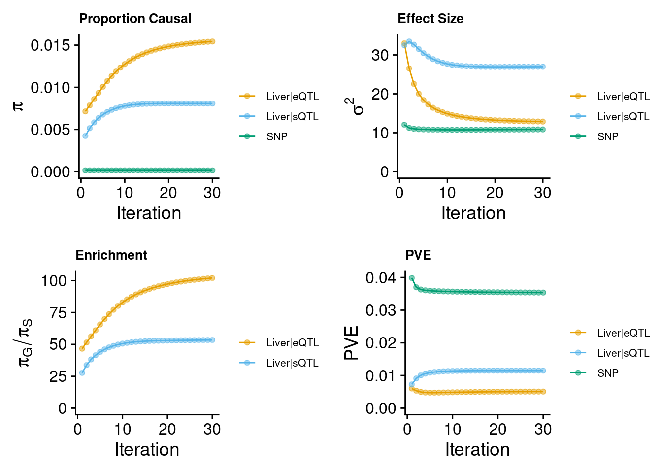
These plots show the estimated prior inclusion probability, prior effect size variance, enrichment and proportion of variance explained (PVE) over the iterations of parameter estimation.
Then, we use summarize_param(param, gwas_n) to obtain
estimated parameters (from the last iteration) and to compute the PVE by
variants and molecular traits.
[1] "The number of genes/introns/SNPs used in the analysis is:"Liver|eQTL Liver|sQTL SNP
8775 18136 7405450 ctwas_parameters$attributable_pve contains the
proportion of heritability mediated by molecular traits and variants, we
visualize it using pie chart.
data <- data.frame(
  category = names(ctwas_parameters$prop_heritability),
  percentage = ctwas_parameters$prop_heritability
)

# Calculate percentage labels for the chart
data$percentage_label <- paste0(round(data$percentage * 100, 1), "%")

ggplot(data, aes(x = "", y = percentage, fill = category)) +
  geom_bar(stat = "identity", width = 1) +
  coord_polar("y", start = 0) +
  theme_void() +  # Remove background and axes
  geom_text(aes(label = percentage_label),
            position = position_stack(vjust = 0.5), size = 5) +
  scale_fill_manual(values = c("#FF9999", "#66B2FF", "#99FF99")) +  # Custom colors
  labs(fill = "Category") +
  ggtitle("Percent of heritability")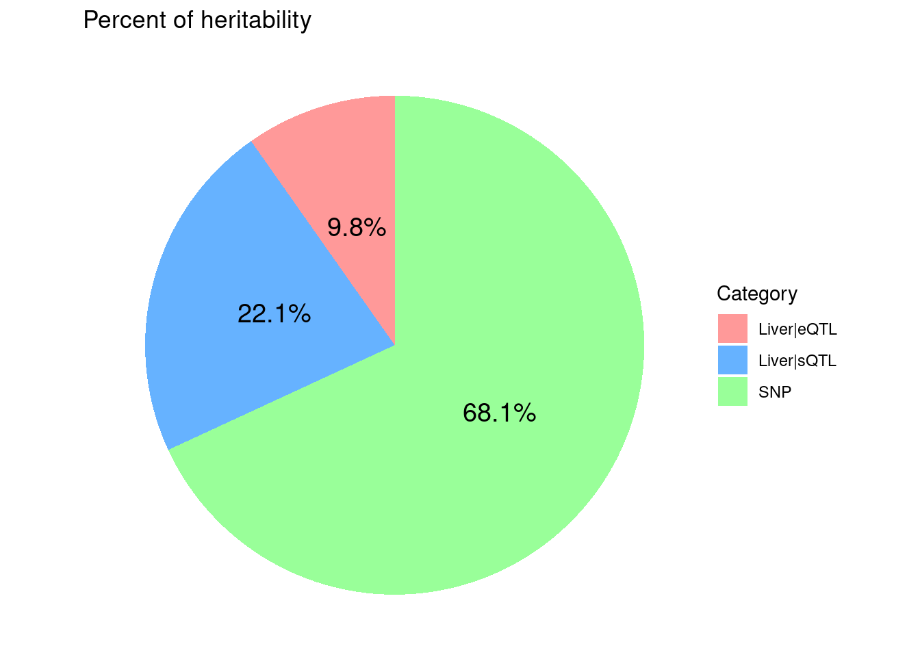
Diagnosis plots
For all genes analyzed, we compare the z-scores and fine-mapping PIPs. We generally expect high PIP molecular traits to have high Z-scores as well. If this is not the case, it may suggest problems, often due to mismatch of reference LD with the LD in the GWAS cohort
finemap_res <- ctwas_res$finemap_res

ggplot(data = finemap_res[finemap_res$type!="SNP",], aes(x = abs(z), y = susie_pip)) +
  geom_point() +
  labs(x = "abs(z-scores)", y = "PIPs") +
  theme_minimal()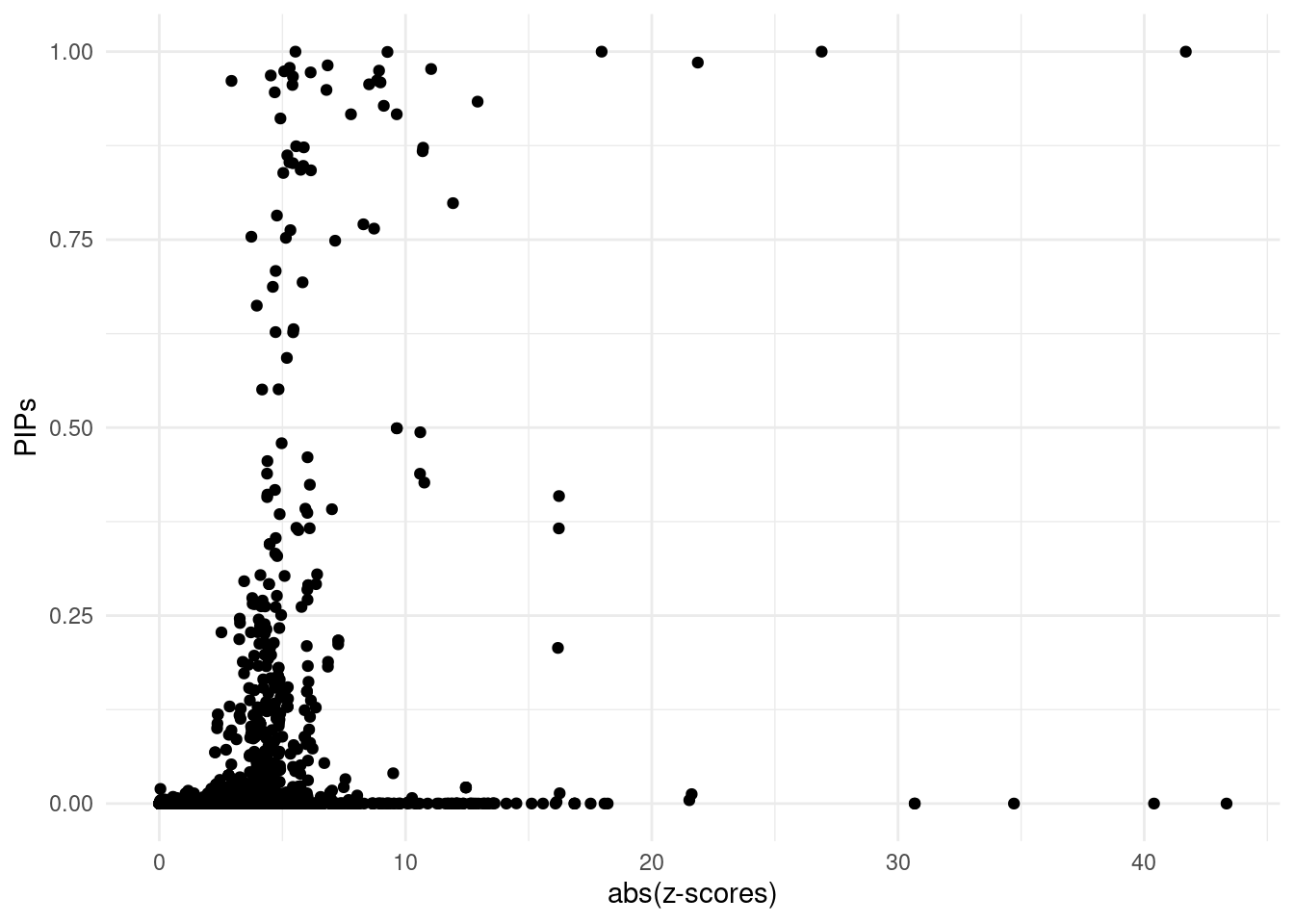
| Version | Author | Date |
|---|---|---|
| 6cf9e49 | XSun | 2024-09-30 |
Fine-mapping results
We process the fine-mapping results here.
We first add gene annotations to cTWAS results
mapping_table <- readRDS("/project2/xinhe/shared_data/multigroup_ctwas/weights/mapping_files/PredictDB_mapping.RDS")

finemap_res$molecular_id <- get_molecular_ids(finemap_res)

snp_map <- readRDS(paste0(results_dir,trait,".snp_map.RDS"))

finemap_res <- anno_finemap_res(finemap_res,
                                         snp_map = snp_map,
                                         mapping_table = mapping_table,
                                         add_gene_annot = TRUE,
                                         map_by = "molecular_id",
                                         drop_unmapped = TRUE,
                                         add_position = TRUE,
                                         use_gene_pos = "mid")
2024-10-14 10:48:06 INFO::Annotating fine-mapping result ...
2024-10-14 10:48:06 INFO::Map molecular traits to genes
2024-10-14 10:48:06 INFO::Split PIPs for molecular traits mapped to multiple genes
2024-10-14 10:48:14 INFO::Add gene positions
2024-10-14 10:48:17 INFO::Add SNP positionsfinemap_res_show <- finemap_res[!is.na(finemap_res$cs) &finemap_res$type !="SNP",]
DT::datatable(finemap_res_show,caption = htmltools::tags$caption( style = 'caption-side: topleft; text-align = left; color:black;','The annotated fine-mapping results, ones within credible sets are shown'),options = list(pageLength = 5) )Next, we compute gene PIPs across different types of molecular traits
library(dplyr)

susie_alpha_res <- ctwas_res$susie_alpha_res

susie_alpha_res <- anno_susie_alpha_res(susie_alpha_res,
                                        mapping_table = mapping_table,
                                        map_by = "molecular_id",
                                        drop_unmapped = TRUE)
2024-10-14 10:48:33 INFO::Annotating susie alpha result ...
2024-10-14 10:48:33 INFO::Map molecular traits to genes
2024-10-14 10:48:33 INFO::Split PIPs for molecular traits mapped to multiple genescombined_pip_by_type <- combine_gene_pips(susie_alpha_res,
group_by = "gene_name",
by = "type",
method = "combine_cs",
filter_cs = TRUE,
include_cs_id = TRUE)
combined_pip_by_type$sQTL_pip_partition <- sapply(combined_pip_by_type$gene_name, function(gene) {
# Find rows in finemap_res_show matching the gene_name
matching_rows <- finemap_res_show %>%
dplyr::filter(gene_name == gene, type == "sQTL") # Match gene_name and filter by type == "sQTL"
# If no matching rows, return NA
if (nrow(matching_rows) == 0) {
return(NA)
}
# Create the desired string format: molecular_id-round(susie_pip, digits = 4)
paste(matching_rows$molecular_id, ":PIP=", round(matching_rows$susie_pip, digits = 4), sep = "", collapse = ", ")
})
DT::datatable(combined_pip_by_type,caption = htmltools::tags$caption( style = 'caption-side: topleft; text-align = left; color:black;','Gene PIPs, only genes within credible sets are shown'),options = list(pageLength = 5) )Locus plots
We make locus plot for the region(“16_71020125_72901251”) containing the gene HPR.
weights <- readRDS(paste0(results_dir,trait,".preprocessed.weights.RDS"))

make_locusplot(finemap_res = finemap_res,
               region_id = "16_71020125_72901251",
               ens_db = ens_db,
               weights = weights,
               highlight_pip = 0.8,
               filter_protein_coding_genes = T,
               filter_cs = T,
               color_pval_by = "cs",
               color_pip_by = "cs")
2024-10-14 10:48:36 INFO::Limit to protein coding genes
2024-10-14 10:48:36 INFO::focal id: ENSG00000261701.6|Liver_eQTL
2024-10-14 10:48:36 INFO::focal molecular trait: HPR Liver eQTL
2024-10-14 10:48:36 INFO::Range of locus: chr16:71020348-72900542chromosome 16, position 71020348 to 729005423650 SNPs/datapoints2024-10-14 10:48:39 INFO::focal molecular trait QTL positions: 72063820,72063928
2024-10-14 10:48:39 INFO::Limit PIPs to credible setsWarning: ggrepel: 31 unlabeled data points (too many overlaps). Consider
increasing max.overlaps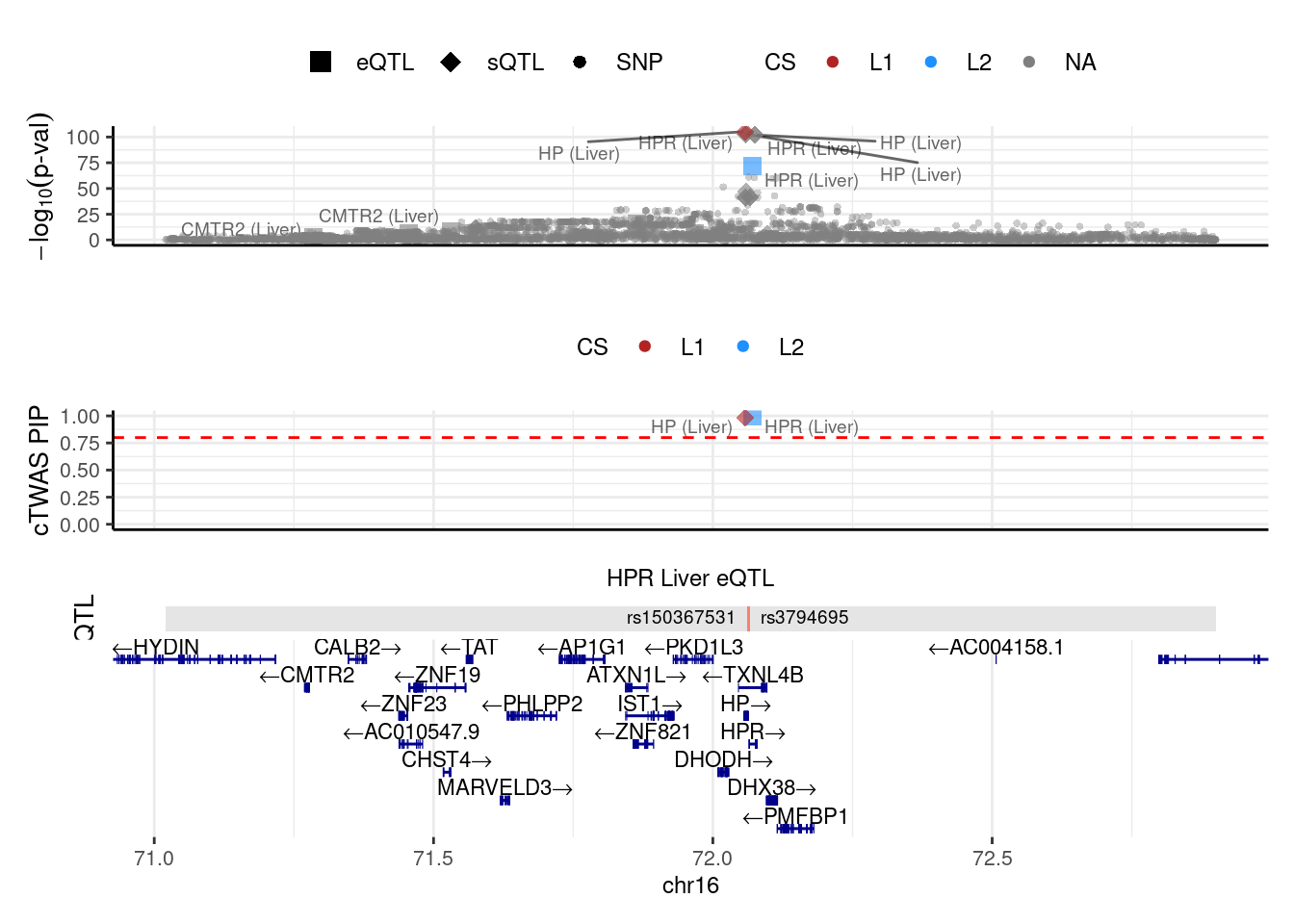
- The top one shows -log10(p-value) of the association of variants (from LDL GWAS) and molecular traits (from the package computed z-scores) with the phenotype
- The next track shows the PIPs of variants and molecular traits. By
default, we only show PIPs of molecular traits and variants in the
credible set(s) (
filter_cs = TRUE) - The next track shows the QTLs of the focal gene.
- The bottom is the gene track.
Gene set enrichment analysis
We do enrichment analysis using the genes with PIP > 0.8
library(enrichR)

dbs <- c("GO_Biological_Process_2021", "GO_Cellular_Component_2021", "GO_Molecular_Function_2021")
genes <- combined_pip_by_type$gene_name[combined_pip_by_type$combined_pip >0.8]

#number of genes for gene set enrichment
sprintf("The number of genes used in enrichment analysis = %s", length(genes))
[1] "The number of genes used in enrichment analysis = 42"GO_enrichment <- enrichr(genes, dbs)Uploading data to Enrichr... Done.
Querying GO_Biological_Process_2021... Done.
Querying GO_Cellular_Component_2021... Done.
Querying GO_Molecular_Function_2021... Done.
Parsing results... Done.print("GO_Biological_Process_2021")[1] "GO_Biological_Process_2021"db <- "GO_Biological_Process_2021"
df <- GO_enrichment[[db]]
print(plotEnrich(GO_enrichment[[db]]))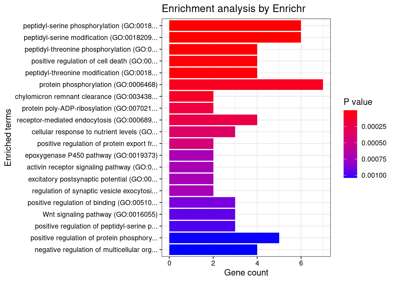
| Version | Author | Date |
|---|---|---|
| 04a6e93 | XSun | 2024-10-10 |
df <- df[df$Adjusted.P.value<0.05,c("Term", "Overlap", "Adjusted.P.value", "Genes")]

DT::datatable(df,caption = htmltools::tags$caption( style = 'caption-side: topleft; text-align = left; color:black;','Enriched pathways from GO_Biological_Process_2021'),options = list(pageLength = 5) )print("GO_Cellular_Component_2021")[1] "GO_Cellular_Component_2021"db <- "GO_Cellular_Component_2021"
df <- GO_enrichment[[db]]
print(plotEnrich(GO_enrichment[[db]]))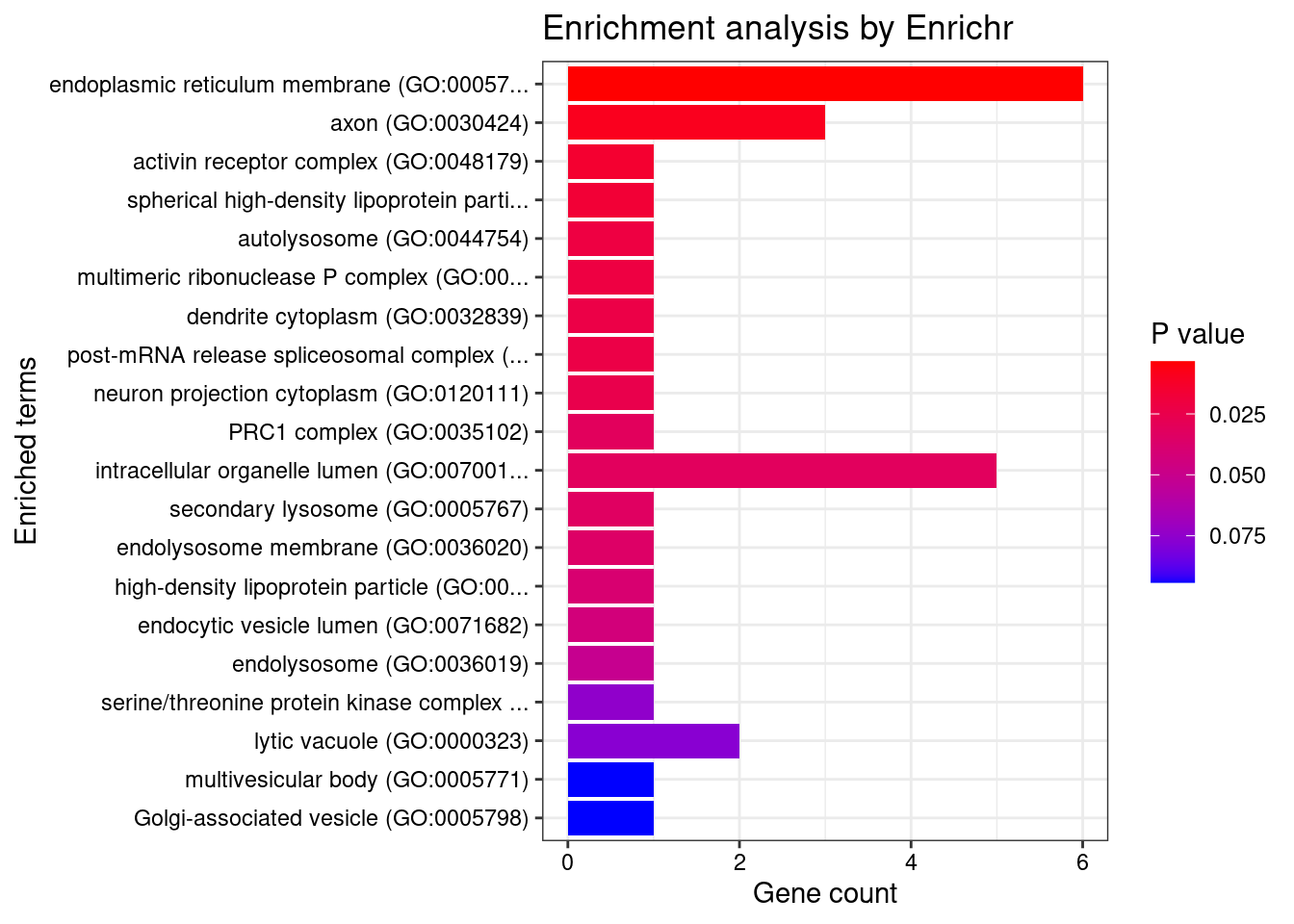
| Version | Author | Date |
|---|---|---|
| 04a6e93 | XSun | 2024-10-10 |
df <- df[df$Adjusted.P.value<0.05,c("Term", "Overlap", "Adjusted.P.value", "Genes")]

DT::datatable(df,caption = htmltools::tags$caption( style = 'caption-side: topleft; text-align = left; color:black;','Enriched pathways from GO_Cellular_Component_2021'),options = list(pageLength = 5) )print("GO_Molecular_Function_2021")[1] "GO_Molecular_Function_2021"db <- "GO_Molecular_Function_2021"
df <- GO_enrichment[[db]]
print(plotEnrich(GO_enrichment[[db]]))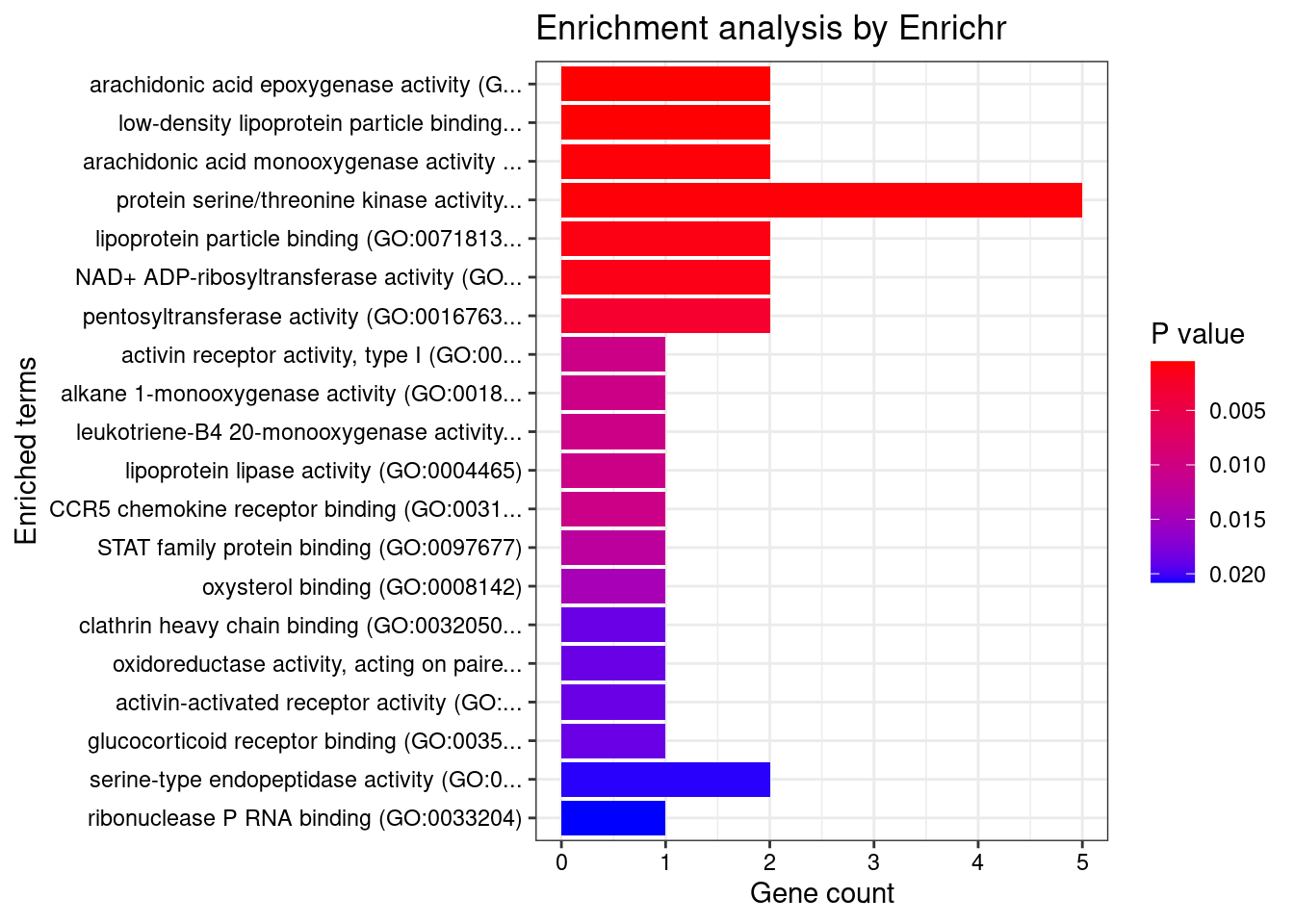
| Version | Author | Date |
|---|---|---|
| 04a6e93 | XSun | 2024-10-10 |
df <- df[df$Adjusted.P.value<0.05,c("Term", "Overlap", "Adjusted.P.value", "Genes")]

DT::datatable(df,caption = htmltools::tags$caption( style = 'caption-side: topleft; text-align = left; color:black;','Enriched pathways from GO_Molecular_Function_2021'),options = list(pageLength = 5) )
sessionInfo()R version 4.2.0 (2022-04-22)
Platform: x86_64-pc-linux-gnu (64-bit)
Running under: CentOS Linux 7 (Core)
Matrix products: default
BLAS/LAPACK: /software/openblas-0.3.13-el7-x86_64/lib/libopenblas_haswellp-r0.3.13.so
locale:
[1] LC_CTYPE=en_US.UTF-8 LC_NUMERIC=C
[3] LC_TIME=en_US.UTF-8 LC_COLLATE=en_US.UTF-8
[5] LC_MONETARY=en_US.UTF-8 LC_MESSAGES=en_US.UTF-8
[7] LC_PAPER=en_US.UTF-8 LC_NAME=C
[9] LC_ADDRESS=C LC_TELEPHONE=C
[11] LC_MEASUREMENT=en_US.UTF-8 LC_IDENTIFICATION=C
attached base packages:
[1] stats4 stats graphics grDevices utils datasets methods
[8] base
other attached packages:
[1] enrichR_3.2 dplyr_1.1.4
[3] ggplot2_3.5.1 EnsDb.Hsapiens.v86_2.99.0
[5] ensembldb_2.20.2 AnnotationFilter_1.20.0
[7] GenomicFeatures_1.48.3 AnnotationDbi_1.58.0
[9] Biobase_2.56.0 GenomicRanges_1.48.0
[11] GenomeInfoDb_1.39.9 IRanges_2.30.0
[13] S4Vectors_0.34.0 BiocGenerics_0.42.0
[15] ctwas_0.4.15
loaded via a namespace (and not attached):
[1] colorspace_2.0-3 rjson_0.2.21
[3] ellipsis_0.3.2 rprojroot_2.0.3
[5] XVector_0.36.0 locuszoomr_0.2.1
[7] fs_1.5.2 rstudioapi_0.13
[9] farver_2.1.0 DT_0.22
[11] ggrepel_0.9.1 bit64_4.0.5
[13] fansi_1.0.3 xml2_1.3.3
[15] codetools_0.2-18 logging_0.10-108
[17] cachem_1.0.6 knitr_1.39
[19] jsonlite_1.8.0 workflowr_1.7.0
[21] Rsamtools_2.12.0 dbplyr_2.1.1
[23] png_0.1-7 readr_2.1.2
[25] compiler_4.2.0 httr_1.4.3
[27] assertthat_0.2.1 Matrix_1.5-3
[29] fastmap_1.1.0 lazyeval_0.2.2
[31] cli_3.6.1 later_1.3.0
[33] htmltools_0.5.2 prettyunits_1.1.1
[35] tools_4.2.0 gtable_0.3.0
[37] glue_1.6.2 GenomeInfoDbData_1.2.8
[39] rappdirs_0.3.3 Rcpp_1.0.12
[41] jquerylib_0.1.4 vctrs_0.6.5
[43] Biostrings_2.64.0 rtracklayer_1.56.0
[45] crosstalk_1.2.0 xfun_0.41
[47] stringr_1.5.1 lifecycle_1.0.4
[49] irlba_2.3.5 restfulr_0.0.14
[51] WriteXLS_6.4.0 XML_3.99-0.14
[53] zlibbioc_1.42.0 zoo_1.8-10
[55] scales_1.3.0 gggrid_0.2-0
[57] hms_1.1.1 promises_1.2.0.1
[59] MatrixGenerics_1.8.0 ProtGenerics_1.28.0
[61] parallel_4.2.0 SummarizedExperiment_1.26.1
[63] LDlinkR_1.2.3 yaml_2.3.5
[65] curl_4.3.2 memoise_2.0.1
[67] sass_0.4.1 biomaRt_2.54.1
[69] stringi_1.7.6 RSQLite_2.3.1
[71] highr_0.9 BiocIO_1.6.0
[73] filelock_1.0.2 BiocParallel_1.30.3
[75] rlang_1.1.2 pkgconfig_2.0.3
[77] matrixStats_0.62.0 bitops_1.0-7
[79] evaluate_0.15 lattice_0.20-45
[81] purrr_1.0.2 labeling_0.4.2
[83] GenomicAlignments_1.32.0 htmlwidgets_1.5.4
[85] cowplot_1.1.1 bit_4.0.4
[87] tidyselect_1.2.0 magrittr_2.0.3
[89] R6_2.5.1 generics_0.1.2
[91] DelayedArray_0.22.0 DBI_1.2.2
[93] withr_2.5.0 pgenlibr_0.3.3
[95] pillar_1.9.0 whisker_0.4
[97] KEGGREST_1.36.3 RCurl_1.98-1.7
[99] mixsqp_0.3-43 tibble_3.2.1
[101] crayon_1.5.1 utf8_1.2.2
[103] BiocFileCache_2.4.0 plotly_4.10.0
[105] tzdb_0.4.0 rmarkdown_2.25
[107] progress_1.2.2 grid_4.2.0
[109] data.table_1.14.2 blob_1.2.3
[111] git2r_0.30.1 digest_0.6.29
[113] tidyr_1.3.0 httpuv_1.6.5
[115] munsell_0.5.0 viridisLite_0.4.0
[117] bslib_0.3.1